MG-RAST user manual¶

Motivation¶

MG-RAST provides Science as a Service for environmental DNA (“metagenomic sequences”) at https://mg-rast.org.

The National Human Genome Research Institute (NHGRI), a division of the National Institutes of Health, publishes information (see Figure [fig:cost_per_megabase]) describing the development of computing costs and DNA sequencing costs over time (Institute 2012). The dramatic gap between the shrinking costs of sequencing and the more or less stable costs of computing is a major challenge for biomedical researchers trying to use next-generation DNA sequencing platforms to obtain information on microbial communities. Wilkening et al. (Wilkening et al. 2009) provide a real currency cost for the analysis of 100 gigabasepairs of DNA sequence data using BLASTX on Amazon’s EC2 service: $300,000. [1] A more recent study by University of Maryland researchers (Angiuoli et al. 2011) estimates the computation for a terabase of DNA shotgun data using their CLOVR metagenome analysis pipeline at over $5 million per terabase.

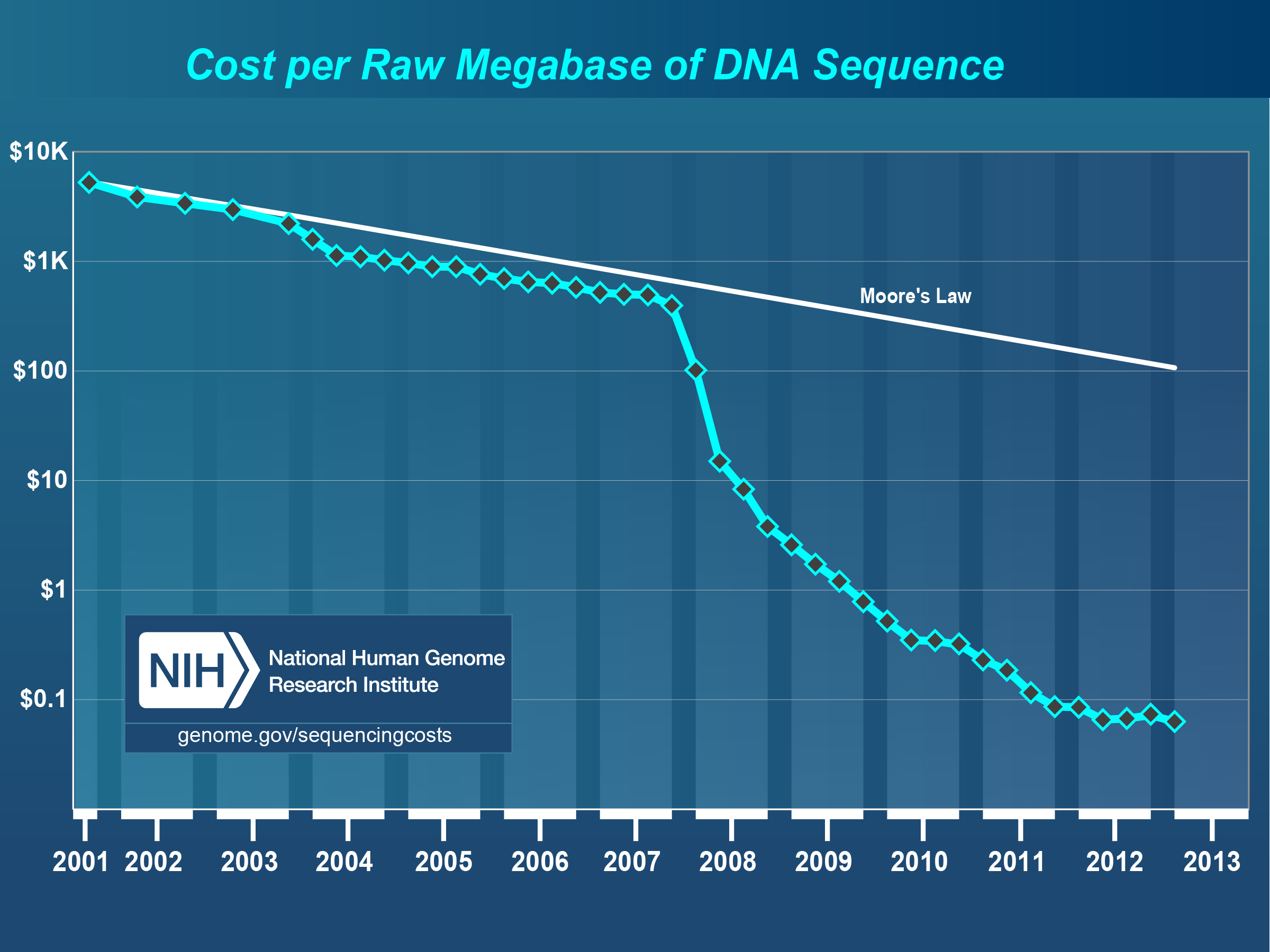
Chart showing shrinking cost for DNA sequencing. This comparison with Moore’s law roughly describing the development of computing costs highlights the growing gap between sequence data and the available analysis resources. Source: NHGRI (Institute 2012)

Nevertheless, the growth in data enabled by next-generation sequencing platforms also provides an exciting opportunity for studying microbial communities: 99% of the microbes in which have not yet been cultured (Riesenfeld, Schloss, and Handelsman 2004). Cultivation-free methods (often summarized as metagenomics) offer novel insights into the biology of the vast majority of life on Earth (Thomas, Gilbert, and Meyer 2012).

Several types of studies use DNA for environmental analyses:

Environmental clone libraries (functional metagenomics): use of Sanger sequencing (frequently) instead of more cost-efficient next-generation sequencing
Amplicon metagenomics (single gene studies, 16s rDNA): next-generation sequencing of PCR amplified ribosomal genes providing a single reference gene–based view of microbial community ecology
Shotgun metagenomics: use of next-generation technology applied directly to environmental samples
Metatranscriptomics: use of cDNA transcribed from mRNA

Each of these methods has strengths and weaknesses (see (Thomas, Gilbert, and Meyer 2012)), as do the various sequencing technologies (see (Loman et al. 2012)).

To support user-driven analysis of all types of metagenomic data, we have provided MG-RAST (Meyer et al. 2008) to enable researchers to study the function and composition of microbial communities. The MG-RAST portal offers automated quality control, annotation, comparative analysis, and archiving services. At the time of writing MG-RAST has completed the analysis of over 100 terabasepairs of DNA data in over 250,000 datasets contributed by thousands of researchers worldwide.

The MG-RAST system provides answers to the following scientific questions:

Who is out there? Identifying the composition of a microbial community either by using amplicon data for single genes or by deriving community composition from shotgun metagenomic data using sequence similarities.
What are they doing? Using shotgun data (or metatranscriptomic data) to derive the functional complement of a microbial community using similarity searches against a number of databases.
Who is doing what? Based on sequence similarity searches, identifying the organisms encoding specific functions.

The system supports the analysis of the prokaryotic content of samples, analysis of viruses and eukaryotic sequences is not currently supported, due to software limitations.

MG-RAST users can upload raw sequence data in fastq, fasta and sff format; the sequences will be normalized (quality controlled) and processed and summaries automatically generated. The server provides several methods to access the different data types, including phylogenetic and metabolic reconstructions, and the ability to compare the metabolism and annotations of one or more metagenomes, individually or in groups. Access to the data is password protected unless the owner has made it public, and all data generated by the automated pipeline is available for download in variety of common formats.

Brief description¶

The MG-RAST pipeline performs quality control, protein prediction, clustering and similarity-based annotation on nucleic acid sequence datasets using a number of bioinformatics tools (see Section 13.2.1. MG-RAST was built to analyze large shotgun metagenomic data sets ranging in size from megabases to terabases. We also support amplicon (16S, 18S, and ITS) sequence datasets and metatranscriptome (RNA-seq) sequence datasets. The current MG-RAST pipeline is not capable of predicting coding regions from eukaryotes and thus will be of limited use for eukaryotic shotgun metagenomes and/or the eukaryotic subsets of shotgun metagenomes.

Data on MG-RAST is private to the submitting user unless shared with other users or made public by the user. We strongly encourage the eventual release of data and require metadata (“data describing data”) for data sharing or publication. Data submitted with metadata will be given priority for the computational queue.

You need to provide (raw or assembled) nucleotide sequence data and sample descriptions (“metadata”). The system accepts sequence data in FASTA, FASTQ and SFF format and metadata in the form or GSC ( http://gensc.org/ ) standard compliant checklists (see Yilmaz et al, Nature Biotech, 2011). Uploads can be put in the system via either the web interface or a command line tool. Data and metadata are validated after upload.

You must choose quality control filtering options at the time you submit your job. MG-RAST provides several options for quality control (QC) filtering for nucleotide sequence data, including removal of artificial duplicate reads, quality-based read trimming, length-based read trimming, and screening for DNA of model organisms (or humans). These filters are applied before the data are submitted for annotation.

The MG-RAST pipeline assigns an accession number and puts the data in a queue for computation. The similarity search step is computationally expensive. Small jobs can complete as fast as hours, while large jobs can spend a week waiting in line for computational resources.

MG-RAST performs a protein similarity search between predicted proteins and database proteins (for shotgun) and a nucleic-acid similarity search (for reads similar to 16S and 18S sequences).

MG-RAST presents the annotations via the tools on the analysis page which prepare, compare, display, and export the results on the website. The download page offers the input data, data at intermediate stages of filtering, the similarity search output, and summary tables of functions and organisms detected.

MG-RAST can compare thousands of data sets run through a consistent annotation pipeline. We also provide a means to view annotations in multiple different namespaces (e.g. SEED functions, K.O. Terms, Cog Classes, EGGnoggs) via the M5Nr.

The publication “Metagenomics-a guide from sampling to data analysis” (PMID 22587947) in Microbial Informatics and Experimentation, 2012 is a good review of best practices for experiment design for further reading.

URL¶

https://mg-rast.org/ http://metagenomics.anl.gov/

License¶

Citing MG-RAST¶

A significant number of papers have been published about MG-RAST
itself and the supporting platform, however we ask that if you use the
system please cite:
The Metagenomics RAST server — A public resource for the automatic
phylogenetic and functional analysis of metagenomes
F. Meyer, D. Paarmann, M. D’Souza, R. Olson , E. M. Glass, M. Kubal,
T. Paczian, A. Rodriguez, R. Stevens, A. Wilke, J. Wilkening, and R.
A. Edwards
BMC Bioinformatics 2008, 9:386

http://www.biomedcentral.com/1471-2105/ 9/386

.

In addition if you also use the API please cite:
A RESTful API for Accessing Microbial Community Data for MG-RAST
A. Wilke, J. Bischof, T. Harrison, T. Brettin, M. D’Souza, W. Gerlach,
H. Matthews, T. Paczian, J. Wilkening, E. M. Glass, N. Desai, F. Meyer
PLOS Comp Biology 2015, DOI: 10.1371/journal.pcbi.1004008

http://journals.plos.org/ploscompbiol/article?id=10.1371/journal.pcbi.1004008

.

Version history¶

Version 1¶

The original version of MG-RAST was developed in 2007 by Folker Meyer, Andreas Wilke, Daniel Paarman, Bob Olson, and Rob Edwards. It relied heavily on the SEED(Overbeek et al. 2005) environment and allowed upload of preprocessed 454 and Sanger data.

Version 2¶

Version 2, released in 2008, had numerous improvements. It was optimized to handle full-sized 454 datasets and was the first version of MG-RAST that was not fully SEED based. Version 2.0 used BLASTX analysis for both gene prediction and functional classification(Meyer et al. 2008).

Version 3¶

While version 2 of MG-RAST was widely used, it was limited to datasets smaller than a few hundred megabases, and comparison of samples was limited to pairwise comparisons. Version 3 is not based on SEED technology; instead, it uses the SEED subsystems as a preferred data source. Starting with version 3, MG-RAST moved to github.

Version 3.6¶

With version 3.6 MG-RAST was containerized, moving from a bare metal infrastructure to a set of docker containers running in a Fleet/SystemD/etcD environment.

Version 4¶

Version 4.0 brings a new web interface, fully relying on the API for data access and moves the bulk of the data stored from Postgres to Cassandra. The new web interface moves the data visualization burden from the web server to the clients machine, using Javascript and HTML5 heavily.

In version 4.0 we have moved the changed the backend store for profiles. While previous version stored a pre-computed mapping of observed abundances to functional or taxonomic categories, this is now computed on the fly. The number of profiles stored is reduced to the MD5 and LCA profiles. The API has been augmented to allow dynamic mapping to categories, to provide the required bandwidth we have migrated the profile store from Postgres to Cassandra.

The web interface of the previous version predated the API, the user interface for version 4.0 now uses the API. The web interface has been re-written in JavaScript/HTML5. Unlike previous version the web interface now is executed on the client (inside the browser) and now soupports any recent browser.

With version 4.04 we are switching the main web site to be mg-rast.org and are also turning on https by default. For a limited time, the unencrypted access protocols will remain available. We encourage all users to upgrade their bookmarks and also install upgraded versions of the CRAN package and/or the python tool suite. We also switched the similarity tool to Diamond(Buchfink, Xie, and Huson 2015).

Comparison of versions 2 and 3¶

Version 3 added the ability to analyze massive amounts of Illumina reads by introducing a significant number of changes to the pipeline and the underlying platform technology. In version 3 we introduced the notion of the API as the central component of the system.

In the 3.0 version, datasets of tens of gigabases can be annotated, and comparison of taxa or functions that differ between samples is now limited only by the available screen real estate. Figure 1.1 shows a comparison of the analytical and computational approaches used in MG-RAST v2 and v3. The major changes are the inclusion of a dedicated gene-calling stage using FragGenescan (Rho, Tang, and Ye 2010), clustering of predicted proteins at 90% identified by using uclust (Edgar 2010), and the use of BLAT (Kent 2002) for the computation of similarities. Together with changes in the underlying infrastructure, this version has allowed dramatic scaling of the analysis with the limited hardware available.

Similar to version 2.0, the new version of MG-RAST does not pretend to know the correct parameters for the transfer of annotations. Instead, users are empowered to choose the best parameters for their datasets.

Comparison of versions 3 and 4¶

The roadmap for version 4 has a number of key elements that will be implemented step-by-step, currently the following features are implemented:

New JavaScript web interface using the API
Cassandra instead of Postgres as main data store for profiles

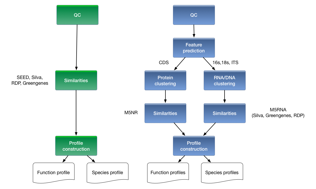
Overview of processing pipeline in (left) MG-RAST v2 and (right) MG-RAST v3. In the old pipeline, metadata was rudimentary, compute steps were performed on individual reads on a 40-node cluster that was tightly coupled to the system, and similarities were computed by BLAST to yield abundance profiles that could then be compared on a per sample or per pair basis. In the new pipeline, rich metadata can be uploaded, normalization and feature prediction are performed, faster methods such as BLAT are used to compute similarities, and the resulting abundance profiles are fed into downstream pipelines on the cloud to perform community and metabolic reconstruction and to allow queries according to rich sample and functional metadata.

The new version of MG-RAST represents a rethinking of core processes and data products, as well as new user interface metaphors and a redesigned computational infrastructure. MG-RAST supports a variety of user-driven analyses, including comparisons of many samples, previously too computationally intensive to support for an open user community.

Scaling to the new workload required changes in two areas: the underlying infrastructure needed to be rethought, and the analysis pipeline needed to be adapted to address the properties of the newest sequencing technologies.

The MG-RAST team¶

MG-RAST was started by Rob Edwards and Folker Meyer in 2007. The MG-RAST team has significantly expanded in the past few years. The team is listed below.

Andreas Wilke
Wolfgang Gerlach
Travis Harrison
William L. Trimble
Folker Meyer

MG-RAST alumni¶

The following people were associated with MG-RAST in the past:

Daniel Paarmann, 2007-2008
Rob Edwards, 2007-2008
Mike Kubal, 2007-2008
Alex Rodriguez, 2007-2008
Bob Olson, 2007-2009
Daniela Bartels, 2007-2011
Yekaterina Dribinsky, 2011
Jared Wilkening, 2007-2013
Mark D’Souza, 2007-2014
Hunter Matthews 2009-2014
Narayan Desai, 2011-2014
Wei Tang, 2012-2015
Daniel Braithwaite, 2012-2015
Elizabeth M. Glass, 2008-2016
Jared Bischof, 2010-2016
Kevin Keegan, 2009-2016
Tobias Paczian 2007 - 2018

Under the hood: The MG-RAST technology platform¶

The backend¶

While originally MG-RAST data was stored in a shared filesystem and a MySQL database, the backend store evolved with growing popularity and demand.

Currently a number of data stores are used to provide the underpinning for various parts of the MG-RAST API.

An approximate mapping of stores to functions in version 4.0 is provided in table [xtab:v4-stores-to-API].

Mapping of API functions to data stores¶
Function	data store	comment
Search	Apache, SOLR and elastic search
Profiles	Cassandra and SHOCK
M5NR	Cassandra
Authentication	MySQL
Project	MySQL
Access control	MySQL
Metadata	MySQL
Files	SHOCK

The backend infrastructure and the overall system layout is shown in figure 2.1.

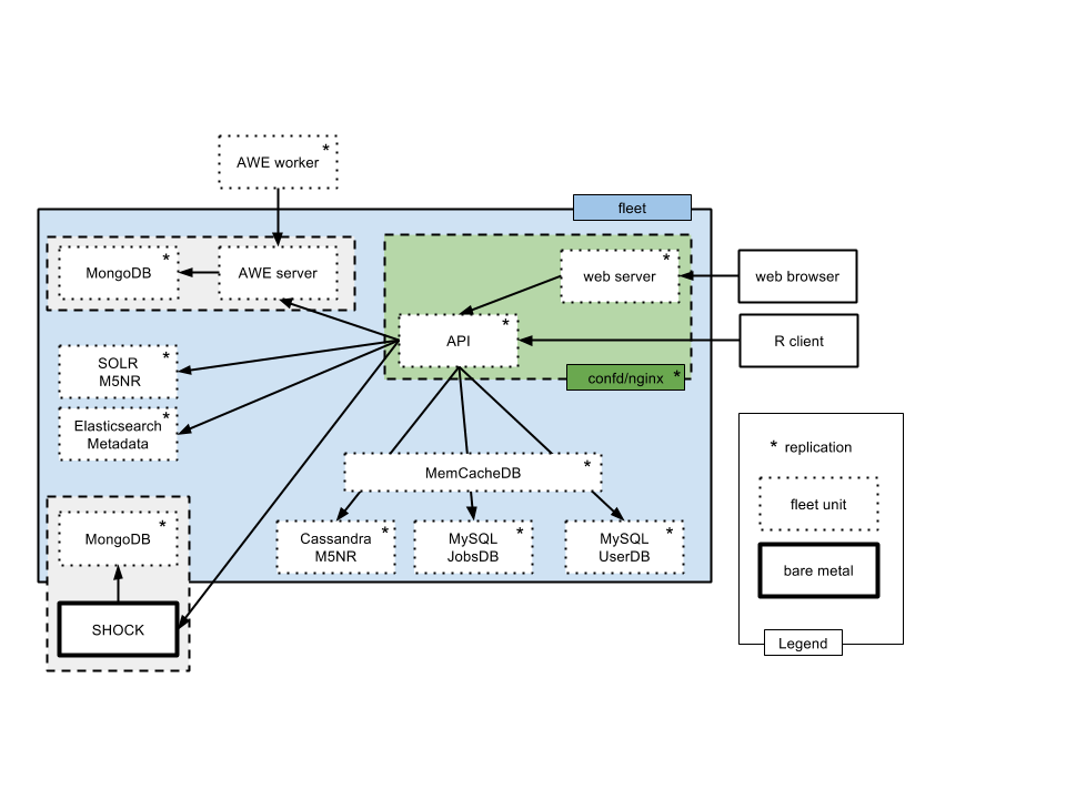
Overview of the production system in mid 2016. Fleet is used to manage a number of containerized services (shown with dashed lines). Two services are provisioned outside the Fleet system: SHOCK (providing 0.7 Petabyte of storage) and a Postgres clusters. We note the significant number of different databases used to serve data required for the API.

As of version 3.6 the majority of the services are provisioned as containers, provisioned as a set of Fleet units described in https://github.com/MG-RAST/MG-RAST-infrastructure/tree/master/fleet-units.

The supporting technologies: Skyport, AWE and SHOCK¶

One key aspect of scaling MG-RAST to large numbers of modern NGS datasets is the use of cloud computing [2], which decouples MG-RAST from its previous dedicated hardware resources.

We use AWE (Wilke et al. 2011) an efficient, open source resource manager to execute the MG-RAST workflow. We expanded AWE to work with Linux containers forming the Skyport system (Gerlach et al. 2014). AWE and Skyport use RESTful interfaces thus allowing the addition of clients without the need to add firewall exceptions and/or massive system reconfiguration.

The main MG-RAST data store is the the SHOCK data management system (Wilke et al. 2015) developed alongside AWE. SHOCK like AWE relies on a RESTful interface instead of a more traditional shared file system.

When we introduced the technologies described above to replace a shared file system (Sun NFS mounted on several hundred nodes), we saw a speed up of a factor of 750x on identical hardware.

Data model¶

The MG-RAST data model (see Figure 2.2) has changed dramatically in order to handle the size of modern next-generation sequencing datasets. In particular, we have made a number of choices that reduce the computational and storage burden.

We note that the size of the derived data products for a next-generation dataset in MG-RAST is typically about 10x the size of the actual dataset. Individual datasets now may be as large as a terabase [3], with the on-disk footprint significantly larger than the basepair count because of the inefficient nature of FASTQ files, which basically double the on-disk size for FASTQ representations.

Abundance profiles. Using abundance profiles, where we count the number of occurrences of function or taxon per metagenomic dataset, is one important factor that keeps the datasets manageable. Instead of growing the dataset sizes (often with several hundred million individual sequences per dataset), the data products now are more or less static in size.
Single similarity computing step per feature type. By running exactly one similarity computation for proteins and another one for rRNA features, we have limited the computational requirements.
Clustering of features. By clustering features at 90% identity, we reduce the number of times we compute on similar proteins. Abundant features will be even more efficiently clustered, leading to more compression for abundant species.

MG-RAST v3 data model.

As shown in Figure 2.2, MG-RAST relies on abundance profiles to capture information for each metagenome. The following abundance profiles are calculated for every metagenome.

MD5s – number of sequences (clusters) per database entry in the M5nr.
functions – summary of all the MD5s that match a given function.
ontologies – summary of all the MD5s that match a given hierarchy entry.
organisms – summary of all MD5s that match a given taxon entry.
lowest common ancestors

The static helper tables (show in blue in Figure [fig:mgrast_analysis-schema]) help keep the main tables smaller, by normalizing and providing integer representations for the entities in the abundance profiles.

THIS NEEDS TO BE REDONE!!!!!!

[fig:mgrast_analysis-schema]

The MG-RAST pipeline¶

Details of the analysis pipeline for MG-RAST version 3

MG-RAST provides automated processing of environmental DNA sequences via a pipeline. The pipeline has multiple steps that can be grouped into five stages:

We restrict the pipeline annotations to protein coding genes and ribosomal RNA (rRNA) genes.

Data hygiene:

Quality control and removal of artifacts.
Feature extraction:

Identification of protein coding and rRNA features (aka “genes”)
Feature annotation:

Identification of putative functions and taxonomic origins for each of the features
Profile generation:

Creation of multiple on disk representations of the information obtained above.
Data loading:

Loading the representations into the appropriate databases.

The pipeline shown in Figure 3.1 contains a significant number of improvements over previous versions and is optimized for accuracy and computational cost.

Using the M5nr (Wilke et al. 2012) (an MD5 nonredundant database), the new pipeline computes results against many reference databases instead of only SEED. Several key algorithmic improvements were needed to support the flood of user-generated data (see Figure [fig:mgrast-job-sizes]). Using dedicated software to perform gene prediction instead of using a similarity-based approach reduces runtime requirements. The additional clustering of proteins at 90% identity reduces data while preserving biological signals.

Below we describe each step of the pipeline in some detail. All datasets generated by the individual stages of the processing pipeline are made available as downloads. Appendix 11 lists the available files for each dataset.

Data hygiene¶

Preprocessing¶

After upload, data is preprocessed by using SolexaQA (Cox, Peterson, and Biggs 2010) to trim low-quality regions from FASTQ data. Platform-specific approaches are used for 454 data submitted in FASTA format: reads more than than two standard deviations away from the mean read length are discarded following (Huse et al. 2007). All sequences submitted to the system are available, but discarded reads will not be analyzed further.

Dereplication¶

For shotgun metagenome and shotgun metatranscriptome datasets we perform a dereplication step. We use a simple k-mer approach to rapidly identify all 20 character prefix identical sequences. This step is required in order to remove Artificial Duplicate Reads (ADRs) (Gomez-Alvarez, Teal, and Schmidt 2009). Instead of simply discarding the ADRs, we set them aside and use them later for error estimation.

We note that dereplication is not suitable for amplicon datasets that are likely to share common prefixes.

DRISEE¶

MG-RAST v3 uses DRISEE (Duplicate Read Inferred Sequencing Error Estimation) (Keegan et al. 2012) to analyze the sets of Artificial Duplicate Reads (ADRs) (Gomez-Alvarez, Teal, and Schmidt 2009) and determine the degree of variation among prefix-identical sequences derived from the same template. See Section 4.2 for details.

Screening¶

The pipeline provides the option of removing reads that are near-exact matches to the genomes of a handful of model organisms, including fly, mouse, cow, and human. The screening stage uses Bowtie (Langmead et al. 2009) (a fast, memory-efficient, short read aligner), and only reads that do not match the model organisms pass into the next stage of the annotation pipeline.

Note that this option will remove all reads similar to the human genome and render them inaccessible. This decision was made in order to avoid storing any human DNA on MG-RAST.

Feature identification¶

Protein coding gene calling¶

The previous version of MG-RAST used similarity-based gene predictions, an approach that is significantly more expensive computationally than de novo gene prediction. After an in-depth investigation of tool performance (Trimble et al. 2012), we have moved to a machine learning approach: FragGeneScan (Rho, Tang, and Ye 2010). Using this approach, we can now predict coding regions in DNA sequences of 75 bp and longer. Our novel approach also enables the analysis of user-provided assembled contigs.

We note that FragGeneScan is trained for prokaryotes only. While it will identify proteins for eukaryotic sequences, the results should be viewed as more or less random.

rRNA detection¶

An initial search using vsearch (???) against a reduced RNA database efficiently identifies ribosomal RNA. The reduced database is a 90% identity clustered version of the SILVA, Greengenes and RDP databases and is used to rapidly identify sequences with similarities to ribosomal RNA.

Feature annotation¶

Protein filtering¶

We indentify possibly protein coding regions overlapping ribosomal RNAs and exclude them from further processing.

AA clustering¶

MG-RAST builds clusters of proteins at the 90% identity level using the cd-hit (???) preserving the relative abundances. These clusters greatly reduce the computational burden of comparing all pairs of short reads, while clustering at 90% identity preserves sufficient biological signals.

Protein identification¶

Once created, a representative (the longest sequence) for each cluster is subjected to similarity analysis.

For rRNA similarities, instead of BLAST we use sBLAT, an implementation of the BLAT algorithm (Kent 2002), which we parallelized using OpenMP (Board 2011) for this work.

As of version 4.04 we have migrated to DIAMOND(Buchfink, Xie, and Huson 2015) to compute protein similarities against M5nr (Wilke et al. 2012). During computation protein and rRNA sequences are represented only via a sequenced derived identifier (an MD5 checksum). Once the computation completes, we generate a number of representations of the observed similarities for various purposes.

Once the similarities are computed, we present reconstructions of the species content of the sample based on the similarity results. We reconstruct the putative species composition of the sample by looking at the phylogenetic origin of the database sequences hit by the similarity searches.

Sequence similarity searches are computed against a protein database derived from the M5nr (Wilke et al. 2012), which provides nonredundant integration of many databases: GenBank,(Benson et al. 2013), SEED (Overbeek et al. 2005), IMG (Markowitz et al. 2008), UniProt (Magrane and Consortium 2011), KEGG (Kanehisa 2002), and eggNOGs (Jensen et al. 2008).

rRNA clustering¶

The rRNA-similar reads are then clustered at 97% identity using cd-hit, and the longest sequence is picked as the cluster representative.

rRNA identification¶

A BLAT similarity search for the longest cluster representative is performed against the M5rna database which integrates SILVA(Pruesse et al. 2007), Greengenes(DeSantis et al. 2006), and RDP(Cole et al. 2003).

Profile generation¶

In the final stage, the data computed so far is integrated into a number of data products. The most important one are the abundance profiles.

Abundance profiles represent a pivoted and aggregated version of the similarity files. We compute best hit, representative hit and LCA abundance profiles (see 4.5).

Database loading¶

In the final step the profiles are loaded into the respective databases.

MG-RAST data products¶

MG-RAST provices a number of data products in a variety of formats.

Fasta and FastQ

Sequence data can be downloaded via the API and web interface as Fasta (or FastQ) files
JSON

Metadata and Tables and other structured data can be downloaded via the APi or the web site in JSON format.
Spreadsheet

Metadata and Tables can be downloaded as spreadsheets via the web interface.
SVG and PNG

Images can be downloaded via the web site interface in SVG and PNG formast.
BIOM v1

BIOM (McDonald et al. 2012) files can be downloaded via the web interface for use with e.g., QIIME (Caporaso et al. 2010).

Sequence data

The originally submitted sequence data as well as the various subsets resulting from processing can be downloaded.
Metadata

data describing data in GSC-compliant format.
Analysis results – results of running the MG-RAST pipeline. The list includes all intermediate data products and is intended to serve as a basis for further analysis outside the MG-RAST pipeline.

Details on the individual files are in Appendix 11.

Abundance profiles¶

Abundance profiles are the primary data product that MG-RAST’s user interface uses to display information on the datasets.

Using the abundance profiles, the MG-RAST system defers making a decision on when to transfer annotations. Since there is no well-defined threshold that is acceptable for all use cases, the abundance profiles contain all similarities and require their users to set cut-off values.

The threshold for annotation transfer can be set by using the following parameters: e-value, percent identity, and minimal alignment length.

The taxonomic profiles use the NCBI taxonomy. All taxonomic information is projected against this data. The functional profiles are available for data sources that provide hierarchical information. These currently comprise the following.

SEED Subsystems

The SEED subsystems(Overbeek et al. 2005) represent an independent reannotation effort that powers, for example, the RAST(Aziz et al. 2008) effort. Manual curation of subsystems makes them an extremely valuable data source.

Subsystems represent a four-level hierarchy:
1. Subsystem level 1 – highest level
2. Subsystem level 2 –
3. Subsystem level 3 – similar to a KEGG pathway
4. Subsystem level 4 – actual functional assignment to the feature in question
The page at http://pubseed.theseed.org/SubsysEditor.cgi allows browsing the subsystems.
KEGG Orthologs

We use the KEGG(Kanehisa 2002) enzyme number hierarchy to implement a four-level hierarchy.
1. KEGG level 1 – first digit of the EC number (EC:X.*.*.*)
2. KEGG level 2 – first two digits of the EC number (EC:X.Y.*.*)
3. KEGG level 3 – first three digits of the EC number (EC:X:Y:Z:.*)
4. KEGG level 4 – entire four digits EC number
We note that KEGG data is no longer available for free download. We thus have to rely on using the latest freely downloadable version of the data.

The high-level KEGG categories are as follows.
1. Cellular Processes
2. Environmental Information Processing
3. Genetic Information Processing
4. Human Diseases
5. Metabolism
6. Organizational Systems
COG and EGGNOG Categories

The high-level COG and EGGNOG categories are as follows.
1. Cellular Processes
2. Information Storage and Processing
3. Metabolism
4. Poorly Characterized
We note that for most metagenomes the coverage of each of the four namespaces is quite different. The “source hits distribution” (see Section [section:source-hits-distribution]) provides information on how many sequences per dataset were found for each database.

DRISEE profile¶

DRISEE (Keegan et al. 2012) is a method for measuring sequencing error in whole-genome shotgun metagenomic sequence data that is independent of sequencing technology and overcomes many of the shortcomings of Phred. It utilizes artificial duplicate reads (ADRs) to generate internal sequence standards from which an overall assessment of sequencing error in a sample is derived. The current implementation of DRISEE is not suitable for amplicon sequencing data or other samples that may contain natural duplicated sequences (e.g., eukaryotic DNA where gene duplication and other forms of highly repetitive sequences are common) in high abundance. DRISEE results are presented on the Overview page for each MG-RAST sample for which a DRISEE profile can be determined. Total DRISEE error presents the overall DRISEE-based assessment of the sample as a percent error:

\[Total \,\, DRISEE \,\, Error = \frac{base\_errors}{total\_bases} * 100\]

where ${base\_errors}$ refers to the sum of DRISEE-detected errors and ${total\_bases}$ refers to the sum of all bases considered by DRISEE. Beneath the Total DRISEE Error, a barchart indicates the error for the sample (the red vertical bar) as well as the minimum (barchart initial value), maximum (barchart final value), mean $(\mu)$, mean +/- one standard deviation ($\sigma$), and mean +/- two standard deviations ($2\sigma$) Total DRISEE Errors observed among all samples in MG-RAST for which a DRISEE profile has been computed.

The DRISEE plot presents a more detailed view of the DRISEE profile; the DRISEE percent error is displayed per base. Individual errors (A,T,C,G, and N substitution rates as well as the InDel rate) are presented as well as a cumulative total.

Users can download DRISEE values as a tab-separated file. The first line of the file contains headers for the values in the second line. The second line contains DRISEE percent error values for A substitutions (A_err), T substitutions (T_err), C substitutions (C_err), G substitutions (G_err), N substitutions (N_err), insertions and deletions (InDel_err), and the Total DRISEE Error. The third line indicates headers for all remaining lines. Rows 4 and 4+ present the DRISEE counts for the indexed position across all considered bins of ADRs. Column values represent the number of reads that match an A,T,C,G,N, or InDel at the indicated position relative to the appropriate consensus sequence followed by the number of reads that do not match an A,T,C,G,N, or InDel.

Kmer profiles¶

kmer digests are an annotation-independent method for describing sequence datasets that can support inferences about genome size and coverage. Here the Overview page presents several visualizations, evaluated at k=15: the kmer spectrum, kmer rank abundance, and ranked kmer consumed. All three graphs represent the same spectrum, but in different ways. The kmer spectrum plots the number of distinct kmers against kmer coverage; the kmer coverage is equivalent to number of observations of each kmer. The kmer rank abundance plots the relationship between kmer coverage and the kmer rank—answering the question “What is the coverage of the nth most-abundant kmer?”. Ranked kmer consumed plots the largest fraction of the data explained by the nth most-abundant kmers only.

Nucleotide histograms¶

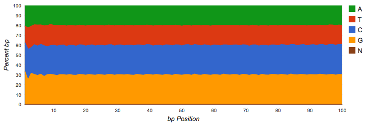
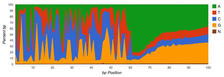
Nucleotide histograms are graphs showing the fraction of base pairs of each type (A, C, G, T, or ambiguous base “N”) at each position starting from the beginning of each read.

Amplicon datasets (see Figure 4.1) should show biased distributions of bases at each position, reflecting both conservation and variability in the recovered sequences:

Nucleotide histogram with biased distributions typical for an amplicon dataset.

Shotgun datasets should have roughly equal proportions of A, T, G and C basecalls, independent of position in the read as shown in Figure 4.2.

Nucleotide histogram showing ideal distributions typical for a shotgun metagenome.

Vertical bars at the beginning of the read indicate untrimmed (see Figure 4.3), contiguous barcodes. Gene calling via FragGeneScan (Rho, Tang, and Ye 2010) and RNA similarity searches are not impacted by the presence of barcodes. However, if a significant fraction of the reads is consumed by barcodes, it reduces the biological information contained in the reads.

Nucleotide histogram with untrimmed barcodes.

If a shotgun dataset has clear patterns in the data, these indicate likely contamination with artificial sequences. The dataset shown in see Figure 4.4 had a large fraction of adapter dimers.

Nucleotide histogram with contamination.

Best hit, representative hit, and lowest common ancestor profiles¶

Mapping the similarities between the predicted protein coding and rRNA sequences to the databases results in files that map the predicted sequences against database entries (“SIM files”). In some cases sequences are identical between different database records, e.g. version of E. coli might share identical proteins and it becomes impossible to determine the “correct” organism name.

In those cases, the translation of those SIMS (that are against an anonymous database, with merely MD5 hashes used as identifiers; see M5NR) can be done in several different ways.

best hit – using one organisms
represenative hit – we pick a random member of the group of idential sequences, the strain you know to be in the sample might not be the representative, the counts are correct, no inflation. (this will ensure that your favorite strain is also listed, but leads to an inflation in the counts)

Figures 4.5 and 4.6 show the effects of using the best and representative hit strategies.

Selecting best hit for mapping data from study mgp128 against Subsystems.

Selecting representative hit for mapping data from study mgp128 against Subsystems leads to inflated numbers.

MG-RAST searches the nonredundant M5nr and M5rna databases in which each sequence is unique. These two databases are built from multiple sequence database sources, and the individual sequences may occur multiple times in different strains and species (and sometimes genera) with 100% identity. In these circumstances, choosing the “right” taxonomic information is not a straightforward process.

To optimally serve a number of different use cases, we have implemented three methods–best hit, representative hit, and lowest common ancestor—for end users to determine the number of hits (occurrences of the input sequence in the database) reported for a given sequence in their dataset.

Best hit¶

The best hit classification reports the functional and taxonomic annotation of the best hit in the M5nr for each feature. In those cases where the similarity search yields multiple same-scoring hits for a feature, we do not choose any single “correct” label. For this reason we have decided to double count all annotations with identical match properties and leave determination of truth to our users. While this approach aims to inform about the functional and taxonomic potential of a microbial community by preserving all information, subsequent analysis can be biased because of a single feature having multiple annotations, leading to inflated hit counts. For users looking for a specific species or function in their results, the best hit classification is likely what is wanted.

Representative hit¶

The representative hit classification selects a single, unambiguous annotation for each feature. The annotation is based on the first hit in the homology search and the first annotation for that hit in our database. This approach makes counts additive across functional and taxonomic levels and thus allows, for example, the comparison of functional and taxonomic profiles of different metagenomes.

Lowest Common Ancestor (LCA)¶

To avoid the problem of multiple taxonomic annotations for a single feature, we provide taxonomic annotations based on the widely used LCA method introduced by MEGAN (Huson et al. 2007). In this method all hits are collected that have a bit score close to the bit score of the best hit. The taxonomic annotation of the feature is then determined by computing the LCA of all species in this set. This replaces all taxonomic annotations from ambiguous hits with a single higher-level annotation in the NCBI taxonomy tree.

Comparison of methods¶

Users should be aware that the number of hits might be inflated if the best hit filter is used or that a favorite species might be missing despite a similar sequence similarity result if the representative hit filter is used (in fact, even if a 100% identical match to a favorite species exists).

One way to consider both the best hit and representative hit is that they overinterpret the available evidence. With the LCA classifier function, on the other hand, any input sequence is classified only down to a trustworthy taxonomic level. While naively this seems to be the best function to choose in all cases because it classifies sequences to varying depths, the approach causes problems for downstream analysis tools that might rely on everything being classified to the same level.

Numbers of annotations vs. number of reads¶

The MG-RAST v3 annotation pipeline does not usually provide a single annotation for each submitted fragment of DNA. Steps in the pipeline map one read to multiple annotations and one annotation to multiple reads. These steps are a consequence of genome structure, pipeline engineering, and the character of the sequence databases that MG-RAST uses for annotation.

The first step that is not one-to-one is gene prediction. Long reads ($>$ $400$bp) and contigs can contain pieces of two or more microbial genes; when the gene caller makes this prediction, the multiple predicted protein sequences (called fragments) are annotated separately.

An intermediate clustering step identifies sequences at 90% amino acid identity and performs one search for each cluster. Sequences that do not fall into clusters are searched separately. The “abundance” column in the MG-RAST tables presents the estimate of the number of sequences that contain a given annotation, found by multiplying each selected database match (hit) by the number of representatives in each cluster. The final step that is not one-to-one is the annotation process itself. Sequences can exist in the underlying data sources many times with different labels. When those sequence are the best hit similarity, we do not have a principled way to choosing the “correct” label. For this reason we have decided to double count these annotations and leave determination of truth to our users. Note: Even when considering a single data source, double-counting can occur depending on the consistency of annotations. Also note: Hits refer to the number of unique database sequences that were found in the similarity search, not the number of reads. The hit count can be smaller than the number of reads because of clustering or larger due to double counting.

Metadata¶

MG-RAST is both an analytical platform and a data integration system. To enable data reuse, for example for meta-analyses, we require that all data being made publicly available to third parties contain at least minimal metadata. The MG-RAST team has decided to follow the minimal checklist approach used by the Genomics Standards Consortium (GSC)(Field et al. 2011).

While the GSC provides a GCDML (R. et al. 2008) encoding, this XML-based format is more useful to programmers than to end users submitting data. We have therefore elected to use spreadsheets to transport metadata. Specifically we use MIxS (Minimum information about any (x) sequence (MIxS) and MIMARKS (Minimum Information about a MARKer gene Survey) to encode minimal metadata (Yilmaz et al. 2010).

The metadata describe the origins of samples and provide details on the generation of the sequence data. While the GSC checklist aims at capturing a minimum of information, MG-RAST can handle additional metadata if supplied by the user. The metadata is stored in a simple key value format and is displayed on the Metagenome Overview page.

Once uploaded, the metadata spreadsheets are validated automatically, and users are informed of any problems.

The presence of metadata enables discovery by end users using contextual metadata. Users can perform searches such as “retrieve soil samples from the continental U.S.A.” If the users have added additional metadata (domain specific extension), additional queries are enabled: for example, “restrict the results to soils with a specific pH”.

The version 4.0 web interface¶

The MG-RAST system provides a rich web user interface that covers all
aspects of the metagenome analysis, from data upload to ordination
analysis. The web interface can also be used for data discovery.
Metadata enables data discovery MG-RAST supports the widely used
MIxS and MIMARKS Standards (Yilmaz, 2011) (as well as domain-specific
plug-ins for specialized environments extending the minimal GSC
standards).
One key aspect of the MG-RAST approach is the creation of smart data
products enabling the user at the time of analysis to determine the
best parameters for, for example, a comparison between samples. This
is done without the need for recomputation of results.
We note that if you want to create links to the MG-RAST web site, you
should use the linkin mechanism instead of linking to any web page
directly. All pages intended for users to create external links
provide the linkin feature, See Section
[section:linkin].

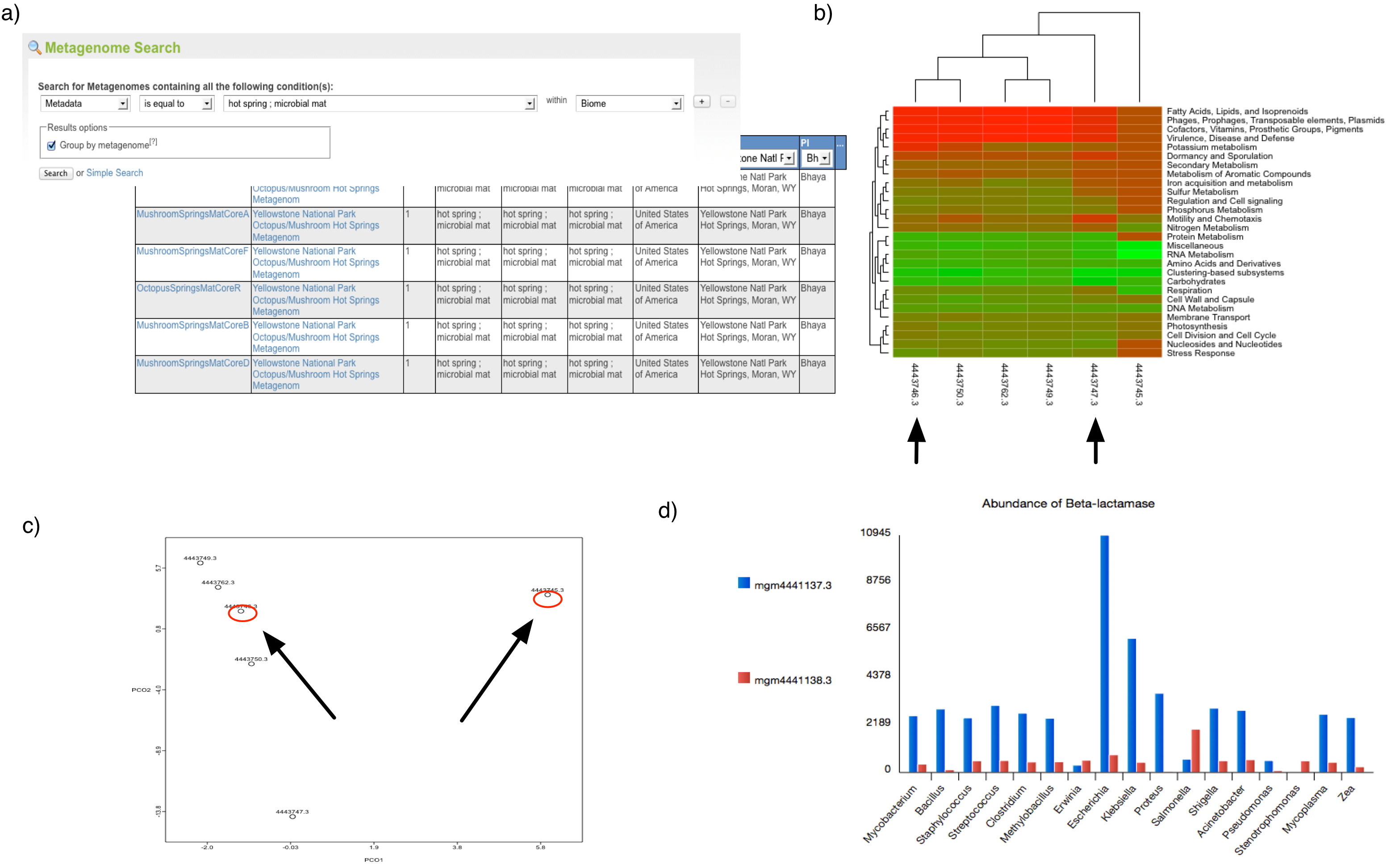
(a) Using the web interface for a search of metagenomes for microbial mats in hotsprings (GSC-MIMS-Keywords Biome=“hotspring; microbial mat”), we find 6 metagenomes (refs: 4443745.3, 4443746.3, 4443747.3, 4443749.3, 4443750.3, 4443762.3). (b) Initial comparison reveals some differences in protein functional class abundance (using SEED subsystens level 1). (c) From the PCoA plot using normalized counts of functional SEED Subsystem–based functional annotations (level 2) and Bray-Curtis as metric, we attempt to find differences between two similar datasets (MG-RAST-IDs: 444749.3, 4443762.3). (d) Using exported tables with functional annotations and taxonomic mapping, we analyze the distribution of organisms observed to contain beta-lactamase and plot the abundance per species for two distinct samples.

Starting with version 4.0 MG-RAST supports an HTML5/JavaScript based web user interface. It supports any recent browser but is tested primarily with Firefox.

Below we are iterating through the various pages in MG-RAST version 4.

Figure 5.1 shows a sample analysis with MG-RAST.

The “My Data” page¶

After login the user is directed to their personal “My Data” page (see figure 5.2), their personal MG-RAST homepage.

This page is provides information on data sets currently being processed, data sets owned by the user as well as any upcoming tasks for the users (i.e. release data to the public after the expiration of the quarantine period).

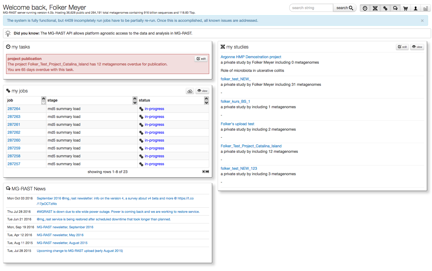
The page shows currently running jobs, the tasks the user needs to perform in the system, a list of their studies and more.

In addition to the data items mentioned above, the page also contains a list of the collections (see [Collections]) owned by the user.

Browsing, searching and viewing studies¶

The search page¶

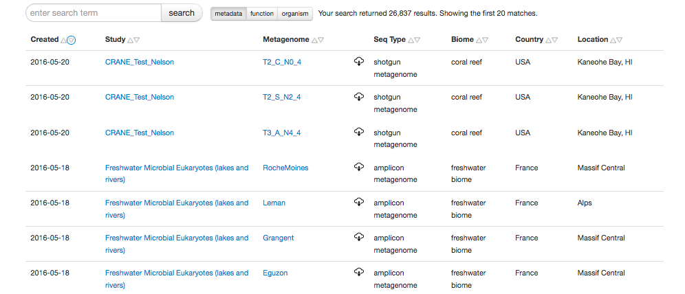
The search page lists all available metagenomic data sets and allows filtering. The looking glass symbol provides access to the search page, there are also shortcuts to the search function on multiple pages.

The basic function of the Search page is to find data sets that (1) contain a search string in the metadata (dataset name, project name, project description, GSC metadata), (2) contain specific functions (e.g., SEED functional roles, SEED subsystems, or GenBank annotations), or (3) contain specific organisms. The default search uses all three kinds of data.

In addition to a Google-like search that searches all data fields, we provide specialized searches in one of the three data types.

We note that due to data visibility (see [section:data-visibility]) not all data sets are visible to all users.

The search page.

The search page has two components, the output widget (see figure 5.3) and the refinement widget.

The refinement widget allows filtering, the creation of saved searches and the creation of collections.

The study page¶

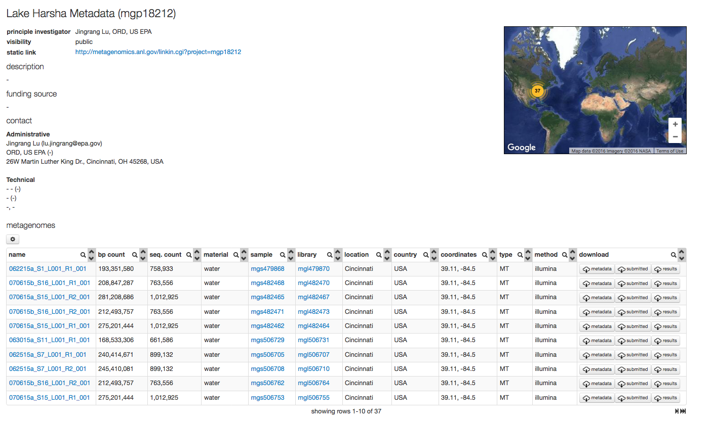
Data in MG-RAST is organized in studies (formerly known as Projects), each study has an automatically generated page.

The study page displays a project title, project description and other study specific information such as funding information. Users are encouraged to provide information on the project in addition to the metadata. The study page also includes the ability to display analysis results generated with the MG-RAST user interface.

A study page.

The study page provides a number of tools to the data set owner:

Sharing

Studies in MG-RAST while initially private (see [section:data-visibility]) can be shared with others. Simply provide any email address for an individual and they will be send a token that allows data access. Sharing is intended to allow pre-publication data sharing.
Reviewer access

Reviewer access tokens can be embedded in Manuscripts (or their cover letters) to allow reviewers and editors access to the data sets.
Data Publication

Data can be made public. This option will generate the only kind of identifiers that should be used in publications.
Metadata editor

Complete or correct the metadata.

Information about specific data sets (Overview page)¶

MG-RAST automatically creates an individual summary page for each dataset. This metagenome overview page provides a summary of the annotations for a single dataset. The page is made available by the automated pipeline once the computation is finished. The page is generated using default values for annotation transfer parameters (e.g. e-values) and thus likely does not represent good biological information, for that please use the Analysis page (see below).

However the Overview page is a good starting point for looking at a particular dataset. It provides a significant amount of information on technical details and biological content.

The page is intended as a single point of reference for metadata, quality, and data. It also provides an initial overview of the analysis results for individual datasets with default parameters. Further analyses are available on the Analysis page.

There are four different types of Overview pages that are displayed as required by the data:

Amplicon metagenome overview page
Shotgun metagenome overview page
Assembled shotgun metagenome overview page
Metatranscriptome overview page

While the different types of overview pages are mostly identical, some visualizations are not relevant or even possible for certain data types. The decision which type of page to display is made based on the data, not the metadata provided by the user.

Previous version of MG-RAST provided almost complete download access to the underlying data, with version 4.0 we have expanded that to all tables and figures. The symbol shown in Figure 5.5.

The download symbol, providing access to the API call and the data in a variety of formats. The (i) displays the API call used to generate the respective data and the pull down menu provides access in variety of formats.

The Overview page provides the MG-RAST ID for a data set, a unique identifier that is usable as accession number for publications. Additional information such as the name of the submitting PI and organization and a user-provided metagenome name are displayed at the top of the page as well. A static URL for linking to the system that will be stable across changes to the MG-RAST web interface is provided as additional information (Figure 5.7).

Please note: Until the data is released to the public, temporary identifiers are made available that will be replaced by permanent valid IDs at the time of data release. The temporary identifiers are long numbers used to represent the data sets until they are public. Do not use temporary identifiers in publications as they are designed to change over time. An example for a temporary ID is 4fbfe5d4216d676d343733343339372e33. A valid MG-RAST identifier is mgm4447101.3. Both the API and the web site work with temporary IDs and MG-RAST IDs.

The results on the Overview page (e.g. link) represent a quick summary of the biological and technical content of each data set. In the past we use a relatively simple approach (best-hit) to compute the biological information. Our reasoning was based on the fact that the “real” meaningful data was presented via the Analysis Page.

With version 4.04 we are now presenting an updated Overview page, results on this page are based on the lowest common ancestor (LCA) algorithm (see Figure 5.6). The LCA (or most recent common ancestor) for a given DNA sequence is computed by evaluating the set of similarities observed when matching the sequence against a number of databases.

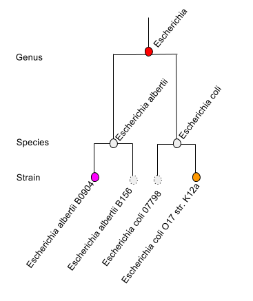
To put this in very simple language, when faced with uncertainty about which species to choose (e.g. when faced with a protein shared by many E. coli species), the MG-RAST Overview page will display a genus level result Escherichia (one level up from species). Likewise if no decision can be made between Escherichia and Shigella (both genera), the LCA will be set to Enterobacteriaceae.

Determining the LCA.

Faced with a decision between multiple strain level hits (purple and orange) for different species, the LCA algorithm will pick higher (genus) level entity.

We note that this will change results for some data sets and cause the analysis pages to look differently, the underlying sequence analysis however is not affected, we merely set a new default value for the generation of overview graphs on this page.

Repeat: The scientific results (presented via the Analysis page) for download or comparison are not affected.

Additional reading: https://en.wikipedia.org/wiki/Most_recent_common_ancestor .

We point the readers attention to the download symbols next to each figure and or table, providing access to the data and API calls underlying each display item.

Top of the metagenome Overview page.

We provide an automatically generated paragraph of text describing the submitted data and the results computed by the pipeline. By means of the project information we display additional information provided by the data submitters at the time of submission or later.

Sequence and feature breakdown¶

One of the first places to look at for each data set are the function and feature breakdown at the top of each overview page.

The pie charts at the top of the overview page (Figure 5.8) classify the submitted sequences submitted into several categories according to their QC results, sequences are classified as having failed QC (grey), containing at least one feature (purple) and unknown if they do not contain any recognized feature (red). In addition the predicted features are broken up into unknown protein (yellow), annotated protein (green) and ribosomal RNA (blue) in a second pie chart.

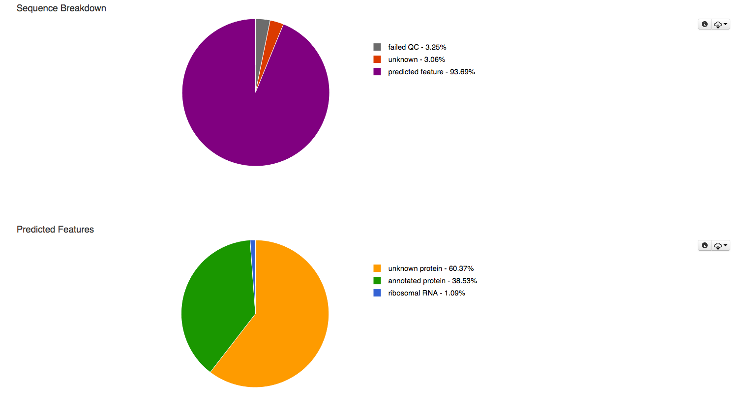
The first pie charts classifies the sequences submitted in this data set according to their QC results, the 2nd breaks down the detected features in to several categories.

What about other feature types?¶

We note that for performance reasons no other sequence features are annotated by the default pipeline. Other feature types such as small RNAs or regulatory motifs (e.g., CRISPRs (Bolotin et al. 2005)) not only will require significantly higher computational resources but also are frequently not supported by the unassembled short reads that constitute the vast majority of todays metagenomic data in MG-RAST. The quality of the sequence data coming from next-generation instruments requires careful design of experiments, lest the sensitivity of the methods is greater than the signal-to-noise ratio the data supports.

Metadata¶

The overview page also provides metadata for each dataset to the extent that such information has been made available. Metadata enables other researchers to discover datasets and compare annotations. MG-RAST requires standard metadata for data sharing and data publication. This is implemented using the standards developed by the Genomics Standards Consortium. Figure 5.9 shows the metadata summary for a dataset.

Information from the GSC MIxS checklist providing minimal metadata on the sample.

All metadata stored for a specific dataset is available in MG-RAST; we merely display a standardized subset in this table. A link at the bottom of the table (“More Metadata”) provides access to a table with the complete metadata. This enables users to provide extended metadata going beyond the GSC minimal standards. A mechanism to provide community consensus extensions to the minimal checklists and the environmental packages are explicitly encouraged but not required when using MG-RAST.

Functional and taxonomic breakdowns¶

A number of pie charts are computed, represening a breakdown of the data into different taxonomic ranks (domain, phylum, class, order, family, genus) an the top levels of the four supported controlled annotation namespaces (Subsystems, Kegg Orthologues (KOGS), COGs and Eggnogs (NOGS)).

Rank abundance¶

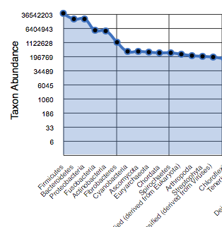
The rank abundance plot (Figure 5.10) provides a rank-ordered list of taxonomic units at a user-defined taxonomic level, ordered by their abundance in the annotations.

Sample rank abundance plot by phylum.

Rarefaction¶

The rarefaction curve of annotated species richness is a plot (see Figure 5.11 of the total number of distinct species annotations as a function of the number of sequences sampled. The slope of the right-hand part of the curve is related to the fraction of sampled species that are rare. On the left, a steep slope indicates that a large fraction of the species diversity remains to be discovered. If the curve becomes flatter to the right, a reasonable number of individuals is sampled: more intensive sampling is likely to yield only few additional species. Sampling curves generally rise quickly at first and then level off toward an asymptote as fewer new species are found per unit of individuals collected.

Rarefaction plot showing a curve of annotated species richness. This curve is a plot of the total number of distinct species annotations as a function of the number of sequences sampled.

The rarefaction curve is derived from the protein taxonomic annotations and is subject to problems stemming from technical artifacts. These artifacts can be similar to the ones affecting amplicon sequencing (Reeder and Knight 2009), but the process of inferring species from protein similarities may introduce additional uncertainty.

Alpha diversity¶

In this section we display an estimate of the alpha diversity based on the taxonomic annotations for the predicted proteins. The alpha diversity is presented in context of other metagenomes in the same project (see Figure 5.12).

$Alpha diversity plot showing the range of :math:`\alpha`-diversity values in the project the data set belongs to. The min, max, and mean values are shown, with the standard deviation ranges (:math:`\sigma` and :math:`2\sigma`) in different shades. The :math:`\alpha`-diversity of this metagenome is shown in red.$

Alpha diversity plot showing the range of $\alpha$-diversity values in the project the data set belongs to. The min, max, and mean values are shown, with the standard deviation ranges ($\sigma$ and $2\sigma$) in different shades. The $\alpha$-diversity of this metagenome is shown in red.

The alpha diversity estimate is a single number that summarizes the distribution of species-level annotations in a dataset. The Shannon diversity index is an abundance-weighted average of the logarithm of the relative abundances of annotated species.

We compute the species richness as the antilog of the Shannon diversity:

\[\textrm{Richness} = 10^{-\sum_i p_i \log(p_i) }\]

where $p_i$ are the proportions of annotations in each of the species categories. Shannon species richness has units of the “effective number of species”. Each $p$ is a ratio of the number of annotations for each species to the total number of annotations. The species-level annotations are from all the annotation source databases used by MG-RAST. The table of species and number of observations used to calculate this diversity estimate can be downloaded under “download source data” on the Overview page.

Functional categories¶

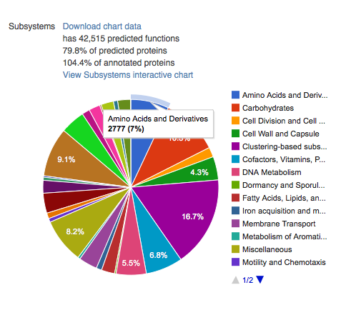
This section contains four pie charts providing a breakdown of the functional categories for KEGG (Kanehisa 2002), COG (Tatusov et al. 2003), SEED Subsystems (Overbeek et al. 2005), and eggNOGs (Jensen et al. 2008). The relative abundance of sequences per functional category can be downloaded as a spreadsheet, and users can browse the functional breakdowns via the Krona tool (Ondov, Bergman, and Phillippy 2011) integrated in the page.

A more detailed functional analysis, allowing the user to manipulate parameters for sequence similarity matches, is available from the Analysis page.

The Subsystems function piechart, showing reads classified into SEED subsystem level-one functions. In contrast to the COG, eggNOG, and KEGG classification schemes, there are over 20 top-level subsystem categories, creating a more highly resolved “fingerprint” for the metagenome.

The sample page¶

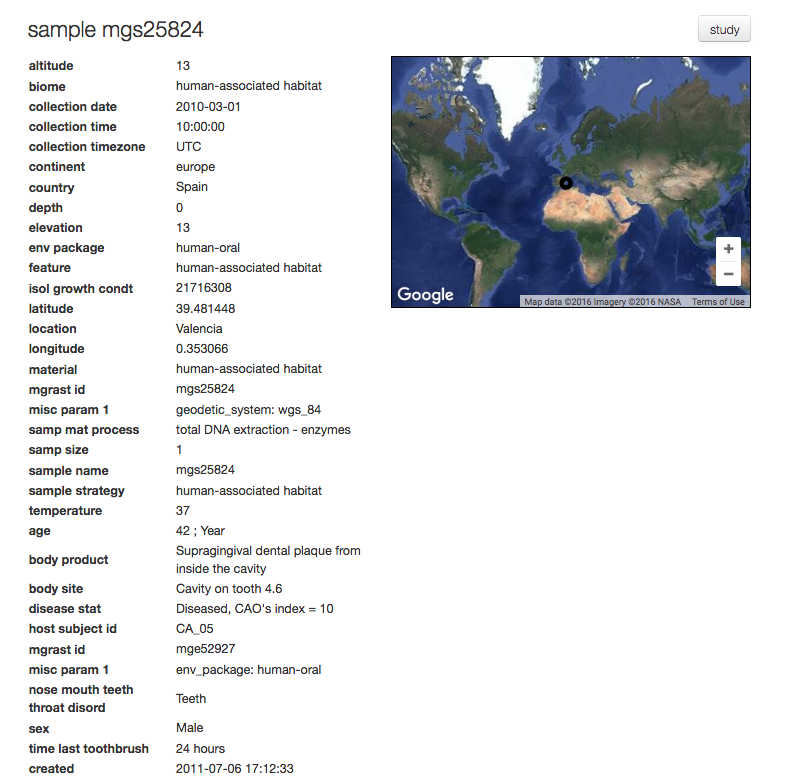
For each sample MG-RAST displays a sample page shown in figure 5.14, the page displays all sample specific information. The information on this page is derived from the metadata.

A sample page.

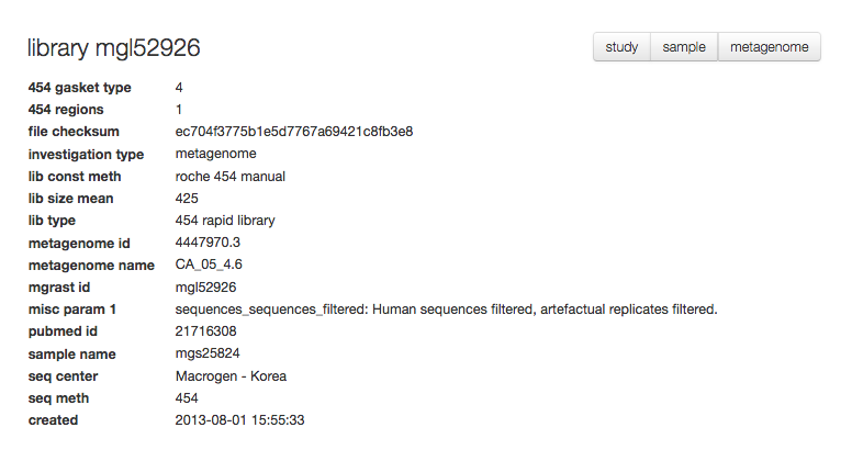
The library page¶

For each set of sequences underlying a data set (“a library”) MG-RAST provides a specific page with information extracted from the metadata.

A library page.

The analysis page – Comparing data, extracting and downloading data¶

The Analysis page is the core of the MG-RAST system, it consumes the various profiles and allows adjusting of parameters.

. It provides a number of tools to compare data sets with different parameters as well as the ability to drill down into the data (e.g. selecting Actinobacteria or features related to a specific functional gene group (e.g. the Lysine Biosynthesis Subsystem).

Compared to previous version of MG-RAST the Analysis page has seen significant improvements, here we provide a step-by-step guide to using the page

Download profiles to local machine for analysis¶

Profiles to be compared, analyzed or visualized need to be downloaded. Figure 5.16 shows an example download of 8 profiles.

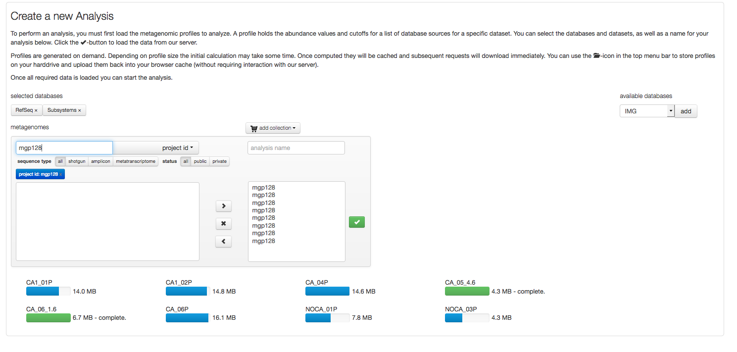
After selecting a project (“mgp128”) the Refseq and Subsystem profiles for the respective data sets are loaded. Blue progress bars indicated profiles being uploaded, green bars indicate the download has completed.

After the profiles have been downloaded, the analysis is no longer dependent on the MG-RAST server resources, instead using the computer the browser is running on. This is achieved via the JavaScript functionality in your browser (please make sure its enabled). Also data is stored in memory, providing you with a good reason to maximize the memory (RAM) of the machine you are running the analysis on.

Normalization¶

Normalization refers to a transformation that attempts to reshape an underlying distribution. MG-RAST now uses DEseq, which is an R package to analyse count data from high-throughput sequencing assays. DESeq, as it has been shown to outperform other methods of normalization - in particular, those that use any sort of linear scaling.

Standardization is a transformation applied to each distribution in a group of distributions so that all distributions exhibit the same mean and the same standard deviation. This removes some aspects of intersample variability and can make data more comparable. This sort of procedure is analogous to commonly practiced scaling procedures but is more robust in that it controls for both scale and location.

The Analysis page calculates the ordination visualizations with either raw or normalized counts, at the user’s option. The normalization procedure is as follows.

$normalized\_value\_i = log2(raw\_counts\_i + 1)$

The standardized values then are calculated from the normalized values by subtracting the mean of each sample’s normalized values and dividing by the standard deviation of each sample’s normalized values.

$standardized\_i = (normalized\_i - mean(normalized\_i)) / stddev(normalized\_i)$

More about these procedures is available in a number of texts. We recommend Terry Speed’s “Statistical Analysis of Gene Expression in Microarray Data” (Speed 2003).

When data exhibit a nonnormal, normal, or unknown distribution, nonparametric tests (e.g., Man-Whitney or Kurskal-Wallis) should be used. Boxplots are easy to use, and the MG-RAST analysis page provides boxplots of the standardized abundance values for checking the comparability of samples (Figure 5.17).

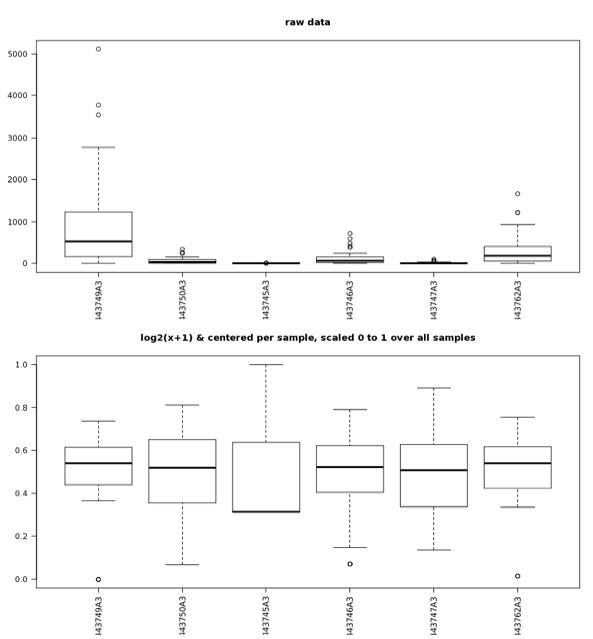
Boxplots of the abundance data for raw values (top) as well as values that have undergone the normalization and standardization procedures (bottom) described in the text. After normalization and standardization, samples exhibit value distributions that are much more comparable and that have a normal distribution; the normalized and standardized data are suitable for analysis with parametric tests; the raw data are not.

Rarefaction¶

The rarefaction view is available only for taxonomic data. The rarefaction curve of annotated species richness is a plot (see Figure 5.18) of the total number of distinct species annotations as a function of the number of sequences sampled. As shown in Figure 5.18, multiple data sets can be included.

The slope of the right-hand part of the curve is related to the fraction of sampled species that are rare. When the rarefaction curve is flat, more intensive sampling is likely to yield only a few additional species. The rarefaction curve is derived from the protein taxonomic annotations and is subject to problems stemming from technical artifacts. These artifacts can be similar to the ones affecting amplicon sequencing (Reeder and Knight 2009), but the process of inferring species from protein similarities may introduce additional uncertainty.

On the Analysis page the rarefaction plot serves as a means of comparing species richness between samples in a way independent of the sampling depth.

Rarefaction plot showing a curve of annotated species richness. This curve is a plot of the total number of distinct species annotations as a function of the number of sequences sampled.

On the left, a steep slope indicates that a large fraction of the species diversity remains to be discovered. If the curve becomes flatter to the right, a reasonable number of individuals is sampled: more intensive sampling is likely to yield only a few additional species.

Sampling curves generally rise very quickly at first and then level off toward an asymptote as fewer new species are found per unit of individuals collected. These rarefaction curves are calculated from the table of species abundance. The curves represent the average number of different species annotations for subsamples of the the complete dataset.

KEGG mapper¶

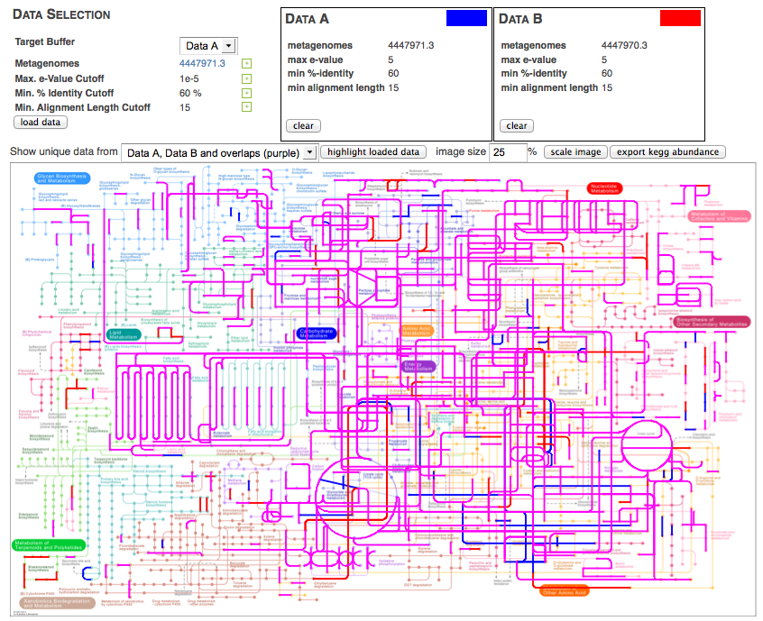
The KEGG map tool allows the visual comparison of predicted metabolic pathways in metagenomic samples. It maps the abundance of identified enzymes onto a KEGG (Kanehisa 2002) map of functional pathways; note that the mapper is available only for functional data). Users can select from any available KEGG pathway map. Different colors indicate different metagenomic datasets.

The KEGG mapper works by providing two buffers that users can assign datasets to. After loading the buffers with the intended datasets, the KEGG mapper can highlight parts of the KEGG map that are present in the dataset. Several combinations of the two datasets can be displayed, as shown in Figure 5.19. Metagenomes can be assigned into one of two groups, and those groups can be visually compared (see Figure 5.20).

Options available for coloring the KEGG maps.

Comparison of two datasets using the KEGG mapper. Parts of metabolism common are shown in purple; unique to A are in blue; unique to B are in red.

Bar charts¶

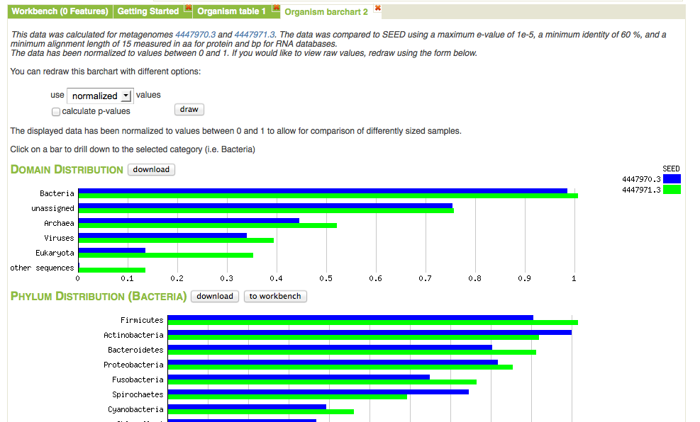
Bar chart view comparing normalized abundance of taxa. We have expanded the Bacteria domain to display the next level of the hierarchy.

Figure 5.21 shows the bar chart visualization option on the Analysis page. One important property of the page is the built-in ability to drill down by clicking on a specific category. In this example we have expanded the domain Bacteria to show the normalized abundance (adjusted for sample sizes) of bacterial phyla. The abundance information displayed can be downloaded into a local spreadsheet. Once a subselection has been made (e.g., the domain Bacteria selected).

Heatmap/Dendrogram¶

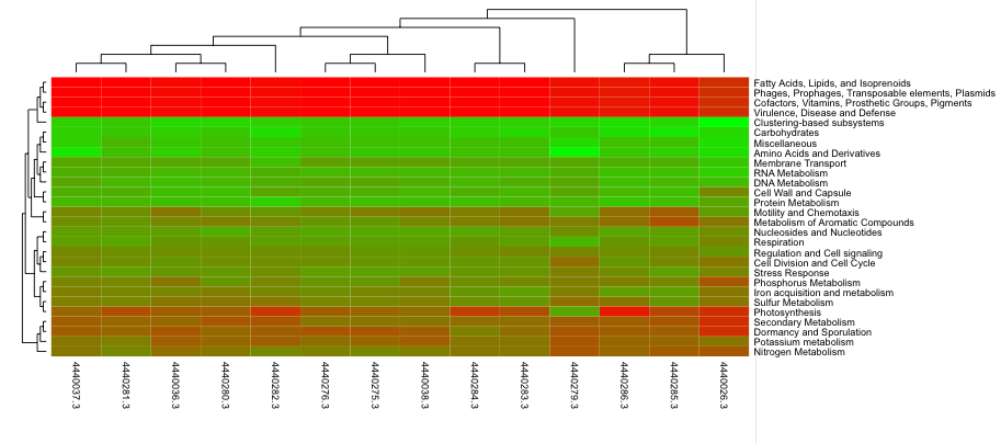
Heatmap/dendogram example in MG-RAST. The MG-RAST heatmap/dendrogram has two dendrograms, one indicating the similarity/dissimilarity among metagenomic samples (x axis dendrogram) and another indicating the similarity/dissimilarity among annotation categories (e.g., functional roles; the y-axis dendrogram).

The heatmap/dendrogram (Figure 5.22) allows an enormous amount of information to be presented in a visual form that is amenable to human interpretation. Dendrograms are trees that indicate similarities between annotation vectors. The MG-RAST heatmap/dendrogram has two dendrograms, one indicating the similarity/dissimilarity among metagenomic samples (x-axis dendrogram) and another indicating the similarity/dissimilarity among annotation categories (e.g., functional roles; the y-axis dendrogram). A distance metric is evaluated between every possible pair of sample abundance profiles. A clustering algorithm (e.g., ward-based clustering) then produces the dendrogram trees. Each square in the heatmap dendrogram represents the abundance level of a single category in a single sample. The values used to generate the heatmap/dendrogram figure can be downloaded as a table by clicking on the download button.

Ordination¶

MG-RAST uses Principle Coordinate Analysis (PCoA) to reduce the dimensionality of comparisons of multiple samples that consider functional or taxonomic annotations. Dimensionality reduction is a process that allows the complex variation found in a large datasets (e.g., the abundance values of thousands of functional roles or annotated species across dozens of metagenomic samples) to be reduced to a much smaller number of variables that can be visualized as simple two- or three-dimensional scatter plots. The plots enable interpretation of the multidimensional data in a human-friendly presentation. Samples that exhibit similar abundance profiles (taxonomic or functional) group together, whereas those that differ are found farther apart.

A key feature of PCoA-based analyses is that users can compare components not just to each other but to metadata recorded variables (e.g., sample pH, biome, DNA extraction protocol) to reveal correlations between extracted variation and metadata-defined characteristics of the samples. It is also possible to couple PCoA with higher-resolution statistical methods in order to identify individual sample features (taxa or functions) that drive correlations observed in PCoA visualizations. This coupling can be accomplished with permutation-based statistics applied directly to the data before calculation of distance measures used to produce PCoAs; alternatively, one can apply conventional statistical approaches (e.g., ANOVA or Kruskal-Wallis test) to groups observed in PCoA-based visualizations.

Table¶

The table tool creates a spreadsheet-based abundance table that can be searched and restricted by the user. Tables can be generated at user-selected levels of phylogenetic or functional resolution. Table data can be visualized by using Krona (Ondov, Bergman, and Phillippy 2011) or can be exported in BIOM(McDonald et al. 2012) format to be used in other tools (e.g., QIIME (Caporaso et al. 2010)). The tables also can be exported as tab-separated text.

Abundance tables serve as the basis for all comparative analysis tools in MG-RAST, from PCoA to heatmap/dendrograms.

Consider the following example showing how to use the taxonomic information derived from an analysis of protein similarities found for the data set 4447970.3. We use the best hit classification, SEED database, $10^{-5}$ evalue, 60% identity, and a minimal alignment length of 15 amino acids. We select table output. The results are shown in Figure 5.23.

The following control elements are connected to the table:

group by – allows summarizing entries below the level chosen here to be subsumed.
download table – downloads the entire table as a spreadsheet.
Krona – invokes KRONA (Ondov, Bergman, and Phillippy 2011) with the table data.
QIIME – creates a BIOM(McDonald et al. 2012) format file with the data being displayed in the table.
table size – changes the number of elements to display for the web page.

View of the analysis page table.

Below we explain the columns of the table and the functions available for them. For each column we allow sorting the table by clicking on the upward- and downward-pointing triangles.

metagenome

In the case of multiple datasets being displayed, this column allows sorting by metagenome ID or selection of a single metagenome.
source

This displays the annotation source for the data being displayed.
domain

The domain column allows subselecting from Archaea, Bacteria, Eukarya, and Viruses.
phylum, class

Since we have selected to group results at the class level, only phylum and class are being displayed. The text fields in the column headers allow subsection (e.g., by entering Acidobacteria or Actinobacteria in the phylum field). The searches are performed inside the web browser and are efficient.

Any subselection will narrow down all datasets being displayed in the table.

Users can elect to have the results grouped by other taxonomy levels (e.g., genus), creating more columns in the table view.
abundance

This indicates the number of sequences found with the parameters selected matching this taxonomic unit. (Note that the parameters chosen are displayed on top of the table.) Clicking on the abundance displays another page displaying the BLAT alignments underlying the assignments.

The abundance is calculated by multiplying the actual number of database hits found for the clusters by the number of cluster members.
avg. evalue, avg percent identity, average alignment length

These indicate the average values for E value, percent identity, and alignment length.
hits

This is the number of clusters found for this entity (function or taxon) in the metagenome.
…

This option allows extending the table to display (or hide) additional columns.

The parameter widget¶

After loading all profiles, the analysis parameter widget is displayed.

Evalue, percent identity, length and minimum abundance filters¶

As shown in Figure 5.25 MG-RAST can changed the parameters for annotation transfer at analysis time. As each data and each analysis is different, we cannot provide a default parameter set for transferring annotations from the sequence databases to the features predicted for the environmental sequence data.

Instead we provide a tool that puts the user at the helm, providing the means to filter the sequences down by selecting only those matching certain criteria.

By changing the e-value, minimum required percent identity or alignment length the annotations to the features loaded, can be modified. We note that the number of hits listed below the filter is reduced and the display is adjusted instanteneously.

*Source type and level filters¶

Adding one or more filters will limit the scope of the sequences analyzed to e.g. a the domain Bacteria (see Figure 5.26). We note that multiple filters can be used and they can be individually erased when no longer needed. Thus the user can filter, e.g. a certain phylum and the identify reads associated with a specific functional gene group.

Adding a domain level filter for Bacteria. The filter is displayed as a blue box and is clearly labeled.

*Example: Display abundance for functional category filtered by taxonomic entities¶

A key feature of the version 4.0 web interface is the ability to filter results. Here we demonstrate filtering results down to the domain Bacteria (Figure 5.27). After the filtering we select COG functional annotations using COG level 2 (Figure 5.28).

The parameter widget allows creation of a Filter for taxonomic units, in this case we use RefSeq annotation to filter at the domain level for Bacteria.

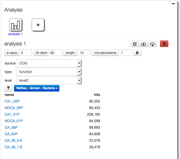
After creating a filter for Bacteria only (using RefSeq taxonomic annotations) we select COG functional annotations using COG level 2.

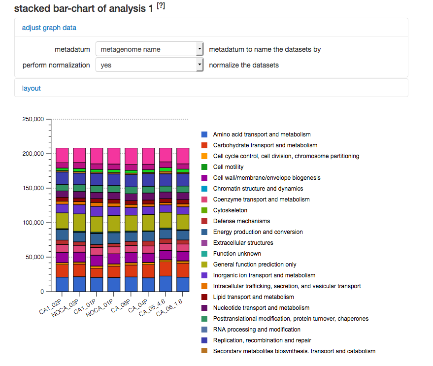
COG level 2 abundance filtered for Bacteria. The results for the settings shown in Figure 5.28

Viewing Evidence¶

For individual proteins, the MG-RAST page allows users to retrieve the sequence alignments underlying the annotation transfers (see Figure 5.30). Using the M5nr (Wilke et al. 2012) technology, users can retrieve alignments against the database of interest with no additional overhead.

BLAT hit details with alignment.

Standard operating procedures SOPs for MG-RAST¶

SOP - Metagenome submission, publication and submission to INSDC via MG-RAST¶

MG-RAST can be used to host data for public access. There are three interfaces for uploading and publishing data, the Web interface, intended for most users, command line scripts, intended for programmers, and the native RESTful API, recommended for experienced programmers.

When data is published in MG-RAST, it can also be released to the INSDC databases. This tutorial covers both use cases.

We note that MG-RAST provides temporary IDs and permanent public identifiers. The permanent identifiers are assigned at the time data is made public. Permanent MG-RAST identifiers begin with “mgm” (e.g. “mgm4449249.3”) for data sets and mgp (e.g.”mgp128”) for projects/studies.

The following data types are supported:

Shotgun metagenomes (“raw” and assembled)
Metatranscriptome data (“raw” and assembled)
Ribosomal amplicon data (16s, 18s, ITS amplicons)
Metabarcoding data (e.g. cytochrome C amplicons; basically all non ribosomal amplicons)

PLEASE NOTE: We strongly prefer raw data over assembled data, if you submit assembled data, please submit the raw reads in parallel. If you perform local optimization e.g. adapter removal or quality clipping, please submit the raw data as well.

This document is intended for experienced to very experienced users and programmers. We recommend that most users not use the RESTful API. There is also a document describing data publication and INSDC submission via the web UI.

An access token for the MG-RAST API, this can be obtained from the MG-RAST web page (http://mg-rast.org) in the user section.

You will need a working python interpreter and the command line scripts and example data can be found in https://github.com/MG-RAST/MG-RAST-Tools:

Scripts: MG-RAST-Tools/tools/bin Data: MG-RAST-Tools/examples/sop/data

Change into MG-RAST-Tools/examples/sop/data and call:

sh get_test_data.sh

to add additional example data.

Either download the repository as a zipped archive from https://github.com/MG-RAST/MG-RAST-Tools/archive/master.zip or use the git command line tool:

git clone http://github.com/MG-RAST/MG-RAST-Tools.git

We tested up to the following parameters:

max. size per file: 10GB
max. project size: 200 metagenomes

While there is no reason to assume the software will not work with larger numbers of files or larger files, we did not test for that.

SOP:¶

Upload and submit sequence data and metadata to MG-RAST using the command mg-submit.py Note: This is an asynchronous process that may take some time depending on the size and number of datasets. (Note: We recommend that novice users try the web frontend; the cmd-line is primarily intended for programmers) The metadata in this example is in Microsoft Excel format, there is also an option of using JSON formatted data. Please note: We have observed multiple problems with spreadsheets that were converted from older version of Excel or “compatible” tools e.g. OpenOffice.

Example:

mg-submit.py submit simple  ....  --metadata

Verify the results and obtain a temporary identifier E.g. by using the WebUI at http://mg-rast.org – you can also use that to publish the data and trigger submission to INSDC.

Publish your project in MG-RAST and obtain a stable and public MG-RAST project identifier

Note: once the data is made public the data is read only, but metadata can be improved

Example:

mg-project make-public $temporary_ID

Trigger release to INSDC/ submit to EBI

Note: Metadata updates are automatically synced with INSDC databases within 48 hours.

Example:

mg-project submit-ebi $PROJECT_ID

Check status of release to INSDC/ submission to EBI

Note: This is an asynchronous process that may take some time depending on the size and number of datasets.

Example:

mg-project status-ebi $PROJECT_ID

We include a sample submission below:

From within the MG-RAST-Tool repository directory

# Retrieve repository and setup environment
git clone http://github.com/MG-RAST/MG-RAST-Tools.git
cd MG-RAST-Tools

# Path to scripts for this example
PATH=$PATH:`pwd`/tools/bin

# set environment variables
source set_env.sh

# Set credentials, obtain token from your user preferences in the UI
mg-submit.py login --token

# Create metadata spreadsheet. Make sure you map your samples to your
# sequence files
# Upload metagenomes and metadata to MG-RAST

mg-submit.py submit simple \
           examples/sop/data/sample_1.fasta.gz \
           examples/sop/data/sample_2.fasta.gz \
           --metadata examples/sop/data/metadata.xlsx

# Output
> Temp Project ID: ed2102aa666d676d343735323836382e33
> Submission ID: 77a1a1a5-4cbd-4673-86bf-f87c9096c3e1

# Remember IDs for later use
SUBMISSION_ID=77a1a1a5-4cbd-4673-86bf-f87c9096c3e1
TEMP_ID=mgp128

# Check if project is finished
mg-submit.py status $SUBMISSION_ID

# Output
> Submission: 77a1a1a5-4cbd-4673-86bf-f87c9096c3e1 Status: in-progress


# Make project public in MG-RAST
mg-project.py make-public $TEMP_ID

# Output
> # Your project is public.
> Project ID: mgp128
> URL: https://mg-rast.org/linkin.cgi?project=mgp128
PROJECT_ID=mgp128

# Release project to INSDC archives
mg-project.py submit-ebi $PROJECT_ID

# Output
> # Your Project mgp128 has been submitted
> Submission ID: 0cf7d811-1d43-4554-ab97-3cb1f5ceb6aa

# Check if project is finished
mg-project.py status-ebi $PROJECT_ID

# Output
> Completed
> ENA Study Accession: ERP104408

REST API uploader¶

The following upload instructions are for using the MG-RAST REST API with the curl program. In order to operate the API the user has to authenticate with an MG-RAST token. The token can be retrieved from the “Account Management” –$>$ “Manage personal preferences” –$>$ “Web Services” –$>$ “authentication key” page via MG-RAST Web site.

We strongly suggest that you use the scripts we provide, instead of the native REST API.

You can upload a file into your inbox with

curl -X POST -H "auth: <myToken>" -F "upload=@<path_to_file>/<file_name>" "https://api.mg-rast.org/inbox"

If you have a compressed file to upload, supports gzip or bzip2

curl -X POST -H "auth: <myToken>" -F "upload=@<path_to_file>/<gzip_file>" -F "compression=gzip" "https://api.mg-rast.org/inbox"
curl -X POST -H "auth: <myToken>" -F "upload=@<path_to_file>/<gzip_file>" -F "compression=bzip2" "https://api.mg-rast.org/inbox"

If you have an archive file containing multiple files to upload do the following two steps, supports: .zip, .tar, .tar.gz, .tar.bz2

1. curl -X POST -H "auth: <myToken>" -F "upload=@<path_to_file>/<archive_file>" "https://api.mg-rast.org/inbox"
2. curl -X POST -H "auth: <myToken>" -F "format=<one of: zip, tar, tar.gz, tar.bz2>" "https://api.mg-rast.org/inbox/unpack/<uploaded_file_id>"

Generating metadata for the submission¶

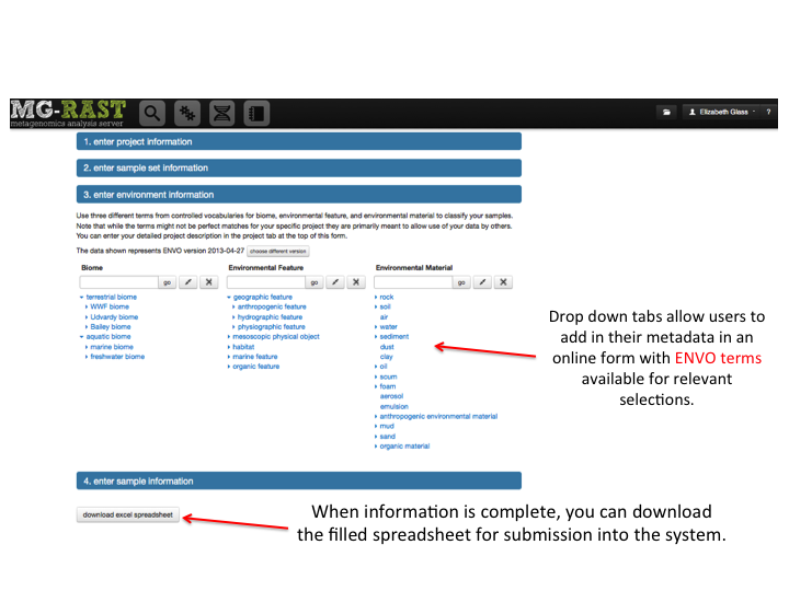
MG-RAST uses questionnaires to capture metadata for each project with one or more samples. Users have two options, they can download and fill out the questionnaire and then submit it or use our online editor, MetaZen. Questionnaires are validated automatically by MG-RAST for completeness and compliance with the controlled vocabularies for certain fields.

MG-RAST has implemented the use of Minimum Information about any (X) Sequence (MIxS)(Yilmaz et al. 2010) developed by the Genomic Standards Consortium. In addition to the minimal checklists, more detailed data can be captured in optional environmental packages.

We use simple spreadsheets to capture metadata, with a minimal number of required fields (in red in the spreadsheets) and a number of optional fields. The spreadsheet is separated into multiple tabs representing the different metadata categories. The MG-RAST metadata spreadsheet template is available on the MG-RAST upload page or at ftp://ftp.mg-rast.org/data/misc/metadata/MGRAST_MetaData_template_1.3.xlsx.

A filled-out version of the spreadsheet is available at ftp://ftp.mg-rast.org/data/misc/metadata/MGRAST_MetaData_template_example.xlsx.

In Figure 9.4 we show the template tab for project and the required field labels (in red) (in essence, your contact information). Figure 9.5 shows the various tabs in the spreadsheet.

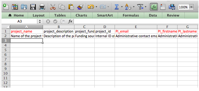
Project spreadsheet. In red are required fields. Note that the 2nd row contains information on how to fill out the form.

The various tabs in the spreadsheet. Project, sample and one of library metagenome or library mimarks survey are required.

Note: Use the third line in the spreadsheet and as shown in Figure 9.6 to enter your data. Do not attempt to alter the first two lines or delete them; they are read only. The first line contains the field labels, and the second line contains descriptions that can help explain how to fill out the fields, along with what unit to use (e.g., temperature in Celsius and distance in meters), URL for the bioportal ontology site etc..

Sample tab with 3 new samples (sample1, sample2, and sample3) added. Again red text in the first row indicates required fields. Rows 1 and 2 cannot be altered.

Required sheets

You need to fill out four sheets to describe your metadata:

Project – This sheet has only one row, and describes a set of samples uploaded together; the other sheets have one row per sample.
Sample – This sheet includes either the filename or metagenome name used for matching.
Library – This sheet includes either the metagenome (for WGS and WXS), mimarks-survey (for 16s and amplicon) or metatranscriptome.
Environmental package (ep) – Several packages of suggested standard metadata are available. Choose the package that best describes your dataset (e.g., water, human-skin, soil).

Sample sheet

The sample sheet requires minimal information (including the sample name) about where and when the sample was taken. Note that some fields in the spreadsheet must be filled out with terms from a controlled vocabulary or in a certain way. Country and environment (biome, feature, material) fields require entries from curated ontologies, gazetteer and environmental ontology, respectively.

Figure 9.6 shows the sample tab with three new samples (sample1, sample2, and sample3) added. Again red text in the first row indicates required fields.

Mandatory fields

Five fields must be completed.

Country – e.g. United States of America, Netherlands, Australia, Uruguay
Latitude and longitude – e.g. [106.84517, -104.60667], [2842.306:math:’N, 8824.099$'$W], [45.30 N, 73.35 W]
Biome – e.g. small lake biome, urban biome, mangrove biome. This term must be one of the terms from the bioportal ontology (http://bioportal.bioontology.org/ontologies/1069?p=terms&conceptid=ENVO%3A00000428). Terms that are not listed on this site are not valid.
Feature – e.g. city, fish farm, livestock-associated habitat, marine habitat, ocean basin, microbial mat. This term must be one of the terms from the bioportal ontology. Terms that are not listed on this site are not valid.
Material – e.g. air, dust, volcanic soil, saliva, blood, dairy product, surface water, piece of gravel. This term must be one of the terms from the bioportal ontology. Terms that are not listed on this site are not valid.

Library section

The library section captures technical data on the preparation and sequencing done. You should choose the library tab to fill out (“metagenome” for shotgun sequencing, “mimarks-survey” for amplicon or “metatranscriptome”) based on the type of sequencing done. These are separated as different sequencing techniques involving different metadata fields. Each row describes one library for one sample. The required fields are colored red.

The sample_name value in the library sheet must exactly match one of the values used in the sample sheet.

The file_name field holds the filename of the sequence file uploaded, or the filename to use for creating the demultiplexed file if you uploaded a multiplexed sequence file and have barcode sequences in the spreadsheet. This is used for mapping sequence files to metadata.

The metagenome_name field holds the name of the metagenome you are submitting. If the file_name field is empty, the metagenome_name will be used to map metadata to sequence files, in this case it would need to match the uploaded sequence filename without the file extension, e.g. a sequence file “test-sequence.fasta” would be mapped to the metadata in the row which has the metagenome_name value “test-sequence”.

The investigation_type field is required to be “metagenome” for shotgun metagenome samples, “mimarks-survey” for amplicon studies or “metatrascriptome”, reflecting which tab was filled out.

The type of sequencing instrument used is another required field. Values are, for example, Sanger, pyrosequencing, ABI-solid, 454, Illumina, assembled, other.

Again, only a limited number of fields are required. However, the more information you provide, the easier it is for you and others to understand any potential uses of your data and to understand why results appear in a particular way. It might, for example, allow understanding of specific biases caused by technology choices or sampled environments.

Environmental Package (ep) sheet

You can fill out one or more environmental metadata packages. Currently we provide support for the following GSC environmental packages:

Air
Built Environment
Host-associated
Human-associated
Human-oral
Human-skin
Human-gut
Human-vaginal
Microbial mat/biofilm
Miscellaneous natural or artificial environment
Plant-associated
Sediment
Soil
Wastewater sludge
Water

We strongly encourage users to submit rich metadata, but we understand the effort required in providing it. Using the environmental packages (which were designed and are used by practitioners in the respective field) should make it reasonably simple to report the essential metadata required to analyze the data. If there is no environmental package to report metadata for your specific sample, please contact MG-RAST staff: we will work with the GSC(Field et al. 2011) to create the required questionnaire.

Using MetaZen¶

MG-RAST uses a simple spreadsheet with 12 mandatory terms. MetaZen designed to help you fill out your metadata spreadsheet. The metadata you provide, helps us to analyze your data more accurately and helps make MG-RAST a more useful analysis resource for everyone.

This tool will help you get started on completing your metadata spreadsheet by filling in any information that is common across all of your samples and/or libraries. This tool currently only allows users to enter one environmental package for your samples and all samples must have been sequenced by the same number of sequencing technologies with the same number of replicates. This information is entered in tab 2.

Note: If your project deviates from this convention, you must either produce multiple separate metadata spreadsheets or generate your spreadsheet and then edit the appropriate fields manually.

Metazen’s online form allows users to either use an existing project, or add in new information to start a new project (Figure [fig:metazen_form]). Users will expand each tab and fill in their metadata information. One of the benefits to using this form is that it provides compliant ENVO terms to select from to describe your sample, without the cumbersome task of looking them up outside of MG-RAST. Figure [fig:metazen_expanded] shows an example of this for entering in environmental information.

The first tab is for project information where you enter the project name and description as well as PI information, information for the technical contact and cross-references to different analysis tools so that your dataset can be linked across these resources.

What you enter in the second tab (sample set information) will dictate what the next tabs will be. Note: You must submit the information here before proceeding with the rest of the form. Enter the information about your set of samples. First, indicate the total number of samples in your set. Second, tell us which environmental package your samples belong to. Then, indicate how many times each of your samples was sequenced by each sequencing method. Each entry of more than zero for number of shotgun, metatranscriptome or amplicon libraries will produce an additional tab to fill out about your sample (Figure [fig:metazen_step2]. Once you add or change information into this form you will need to press the button “show library input forms” to update subsequent tabs.

Note: It is allowable to indicate here if your samples were sequenced using more than one sequencing method.

Once the data has been entered, click on “download excel spreadsheet” to download your filled sheet. You can now use this for upload and submission to MG-RAST.

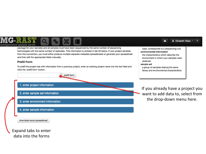
The Metazen form for filling out metadata allows users to fill in data online and add data to existing projects or start new ones. Tabs are expandable and reveal forms for the various required metadata sections.

[fig:metazen_form]

The Metazen form for filling out metadata allows users to fill in data using standard nomenclature.

[fig:metazen_expanded]

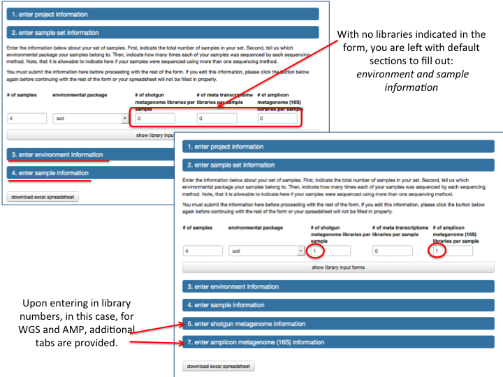
The second tab in the Metazen form must be filled out before moving further down the forms. Selecting the number of libraries (other than zero) adds forms for those libraries. Click on the “show library input forms” button to display them. If no libraries are entered, then only the default tabs for environment and sample information are provided.

[fig:metazen_step2]

Can I upload files to my inbox through the MG-RAST API?¶

Yes. You can upload files to your user inbox using the MG-RAST API with the command-line tool cURL, invoked as:

curl -H "auth: webkey" -X POST -F "upload=@/path_to_file/metagenome.fasta"
          "https://api.mg-rast.org/1/inbox/" > curl_output.txt

where you need to substitute “webkey” with the unique string of text generated by MG-RAST for your account. Your webkey is valid for a limited time period and ensures that the uploads you perform from the command line are recognized as belonging to your MG-RAST account and placed in the correct inbox.

How do I handle the metadata for paired end reads?¶

With paired reads (e.g. R1 and R2) the reads can be merged prior to submission, in this case the metadata should only refer to the new merged reads.

You only need to include metadata for the R1 and R2 reads separately if you choose to treat the second read (R2) as a technical replicate. The mate pair merging can be handled by the Web UI by the submission script we provide in the MG-RAST tools repository. TBA

What type of sequence files should I upload?¶

Your sequence data can be in FASTA, FASTQ or SFF format. These are recognized by the file name extension with valid extensions for the appropriate formats .fasta, .fna, .fastq, .fq, and .sff and FASTA and FASTQ files need to be in plain text ASCII. Compressing large files will reduce the upload time and the chances of a failed upload, you can use gzip (.gz), bzip2 (.bz2) Zip (.zip less than 4 GB in size) as well as tar archives compressed with gzip (.tar.gz) or bzip2 (.tar.bz2), rar files are not accepted. We suggest you upload raw data (in FASTQ or SFF format) and let MG-RAST perform the quality control step, see Section 3 for details.

What type of sequence files should I NOT upload?¶

MG-RAST will not analyze the following:

protein sequences,
WGS reads <75bp,
complete genomes,
sequence data less than 1Mbp,
sequences containing alignment information,
ABIsolid sequences in colorspace,
rar compressed files,
Zip files over 4GB,
Word documents,
Rich Text Format files, and
files without the extension .fna, .fasta, .fq, .fastq or .sff in their name.

How do I prepare my metadata for upload?¶

You can submit metadata for your samples during the upload/submission process. The metadata is transferred to MG-RAST in a spreadsheet in which you can enter metadata for one or more samples along with information about the project the samples should be placed in. Step one in the first section, ‘Prepare data’, has the empty metadata spreadsheet template available for download with the required fields labeled in red. The metadata is hierarchical with three levels, project, sample and library. There has to be a sequence file corresponding to each library entry and the sequence filename must match the library file_name fields or match the library metagenome_name fields minus extension. Once you have filled out the spreadsheet with metadata you can upload it along with the sequence files to your inbox with the MG-RAST uploader.

Will my metadata file in .xls format work OK?¶

Yes, the site is designed to handle .xls metadata files and we have successfully tested uploading and validating .xls files. The metadata template file we provide is a .xlsx file and that is the preferred format If you do experience problems with a .xls file being recognized, Microsoft provides a convertor to the .xslx format:

How are the projects listed on the upload page during submission selected?¶

During the submission process, you can choose to place the new datasets in an existing project. All the projects you have write access to will be listed for selection, this includes all the projects you own as well as projects owned by other users for which you have been granted write access. You can also specify a particular project from this list in the metadata template file or create a new project for your dataset(s) by typing in the name.

How much time will it take to upload my data to MG-RAST?¶

Based on observed values, upload times per 1GB (10:sup:9 bytes) vary from 2 minutes to over an hour with typical times being 10 to 15 minutes. Your experience will vary depending on the speed of your connection to the internet and the quality of service in your region. The fastest times that could be expected for the technology you are using is listed in table [table:upload_speeds]. In practice the time taken will be more than indicated in the table.

Upload speeds for different technologies¶
Technology	Rate	Time for 1GB Upload
Modem 14.4 (2400 baud)	14.4 kbit/s	154 hours
ADSL Lite	1.5 Mbit/s	1.5 hours
Ethernet	10 Mbit/s	13.33 minutes
T3	44.74 Mbit/s	3 minutes
Fast Ethernet	100 Mbit/s	1.33 minutes

[table:upload_speeds]

Do I need to compress my files before uploading to MG-RAST?¶

It is not required that you compress your files before uploading to MG-RAST, but it is highly recommended.

Compressing your sequence data using Zip or gzip before it is uploaded will reduce the time required for the upload. The compression rate depends on the nature of the sequences, typical compression rates for uploaded sequence data that we have observed is between 30-35%. This means the time taken for the upload may be reduced by a third or even more. On a slow connection where uploading 1GB takes over an hour this could be a considerable reduction in time. In addition, the shortened time will also reduce the chance of a failed upload if something goes wrong.

What does the “Join paired-ends” function do?¶

The ‘Join paired-ends’ function on the Upload page allows users to merge two fastq files which represent paired end reads from the same sequencing run. The fastq-join utility (http://code.google.com/p/ea-utils/wiki/FastqJoin) is used to merge mate-pairs with a minimum overlap setting of 8bp and a maximum difference of 10% (parameters: -m 8 -p 10). There is an option to retain or remove the pairs which do not overlap—the ‘remove’ option drops paired reads for which no overlap is found and the ‘retain’ option will keep non-overlapping paired reads in your output file as separate individual (non-joined) sequences. There is also an option to include an index file (if you have one) that contains the barcode for each mate-pair. If this file is included, the barcodes will be reverse-complemented and then prepended to the output sequences.

What does the “assembled” pipeline option do?¶

The “assembled” pipeline option allows users to submit sequence data under a slightly altered analysis pipeline that is more appropriate for assembled sequences. Your assembled contigs should be uploaded in FASTA format and should include the abundance of each contig in your dataset with the following format:

>sequence_number_1_[cov=2]
CTAGCGCACATAGCATTCAGCGTAGCAGTCACTAGTACGTAGTACGTACC...
>sequence_number_2_[cov=4]
ACGTAGCTCACTCCAGTAGCAGGTACGTCGAGAAGACGTCTAGTCATCAT...

The abundance information must be appended without spaces to the end of the sequence name (also without whitespace) in the format

_[cov=n]

where ‘n’ is the coverage or abundance of each contig.

Can I use the coverage information in my Velvet sequence file?¶

Yes, coverage information can be included in the header lines of FASTA-formatted files, for the exact format see the FAQ entry on the assembled pipeline.

The following unix command:

cat contigs.fa |
   sed 's/_cov_\([0-9]*\).[0-9]*/_[cov=\1]/;' > Assembly-formatted-for-MGRAST.fa

should transform Velvet’s default FASTA output into MG-RAST’s preferred output.

Adding one more term:

cat contigs.fa |
     sed 's/_cov_\([0-9]*\).[0-9]*/_[cov=\1]/;
          s/NODE/Assembly-and-sample-name/' > Assembly-formatted-for-MGRAST.fa

will give the contigs better names than NODE_4_etc., substitute your information for ’Assembly-and-sample-name’.

Job processing¶

How long does it take to analyze a metagenome?¶

The answer depends on three factors:

the priority assigned to your dataset,
the size of your dataset, and
the current server load.

In practice the time taken will range between a few hours and a week.

How is the job processing priority assigned?¶

MG-RAST assigns a priority to each dataset which will influence the order in which datasets are selected for processing as well as the processing speed for individual stages in the analysis pipeline. The priority of processing a dataset is based on its usefulness to the scientific community and is estimated using a combination of the amount of metadata supplied and the length of time before the dataset will be made public. The highest priority is given to datasets with complete metadata that will be made public immediately.

Analysis pipeline¶

How is the dereplication step performed?¶

The dereplication step is performed to remove replicates which can be produced during sequencing. MG-RAST identifies two reads as replicates if they have 100% identity over the first 50 basepairs. This step is optional and you should skip it for amplicon data.

What does the “demultiplex” function do?¶

The ‘demultiplex’ function on the Upload page gives users the ability to demultiplex a multiplexed sequence file. The user enters the multiplexed sequence file and a bar codes file. A process is then run that separates out sequences, based upon bar codes, into separate sequence files. The separate sequence files are then turned into separate jobs in MG-RAST upon submission..

How is the job processing priority assigned?¶

MG-RAST assigns a priority to each dataset which will influence the order in which datasets are selected for processing as well as the processing speed for individual stages in the analysis pipeline. The priority of processing a dataset is based on its usefulness to the scientific community and is estimated using a combination of the amount of metadata supplied and the length of time before the dataset will be made public. The highest priority is given to datasets with complete metadata that will be made public immediately.

Analysis results¶

What annotations does MG-RAST display?¶

At the moment, the annotations provided by MG-RAST are annotations produced by the MG-RAST v3.2 analysis pipeline. Different pipelines (and different pipeline strategies) may produce different results, and the results of different annotation strategies are notoriously different to reconcile. Some users have reported and published using annotations that differ from those produced by MG-RAST; we provide the MG-RAST annotations. While in theory the various annotation tools and approaches do similar things (annotating reads based on similarity to sequences in the public databases), the various approaches can provide significantly different descriptions, particularly at the species level.

Why don’t the numbers of annotations add up to the number of reads?¶

See Section 4.6.

Is the alignment length in amino acids or in nucleotides?¶

For the protein similarities against the protein databases, alignment length is in amino acids. For the nucleic acid similarities against the RNA databases, the alignment length is in nucleotides.

Why am I seeing RNA similarities in my shotgun dataset?¶

MG-RAST identifies sequences similar to known RNA sequences in shotgun data and annotates them in addition to providing protein function annotation and protein-derived taxonomic annotation. Your mileage may vary.

Why am I seeing protein similarities in my RNA dataset?¶

These are called “false positives”. We fall back on human judgment when computers give results that don’t make sense.

Why don’t you suppress the false positives?¶

If we suppress protein similarities when we think a dataset is RNA, we will sometimes make mistakes, and suppress protein similarities on a dataset that is, say, a metatranscriptome, for which the protein similarities are the principal objective. These might be called “false negatives”, and our users don’t want that.

What do all those symbols in the similarities table mean?¶

The MG-RAST system was designed to annotate large datasets; the similarities output is designed for the convenience of the MG-RAST system and not the end user. MG-RAST uses 32-character symbols like this 28614b98db4f4efc13b8b20b21ee9b95 (md5 protein identifiers) as the labels for protein sequences, regardless of database.

Can I run a BLAST search against all public metagenomes?¶

No. Such a search is too computationally expensive. But you can find public metagenomes that contain proteins that hit your favorite sequence from the Search page.

Download¶

Where is the table of reads with the annotation for each read?¶

MG-RAST versions 1 and 2 had this type of output, but MG-RAST v3 does not. MG-RAST version 3 has been optimized for large (Gbase+) datasets, and per-read annotation for large datasets is extremely bulky and difficult to interpret. The per-read annotations are not stored in a file on the server, but can be downloaded using the MG-RAST API.

Where can I download the results of the metagenome analysis?¶

Every completed MG-RAST dataset has a page where you can download the files produced by the different stages of the analysis, click on the link on the metagenome overview page. Datasets which have been made public have links to an ftp site at the top of this download page where you can access additional information.

How do I download everything?¶

As of April 2014 we have over 7 x 10¹² bases of public sequence data, so you might want to consider if all the data is really what you need to answer your research question.

Public datasets, including sequence data and annotation data products, are available from our API.

Privacy¶

Who can access my uploaded data?¶

Your uploaded data will remain confidential as long as you do not share it with other users. You will have the ability to share the data with individuals or publish it to the MG-RAST community.

Will my private jobs ever be deleted?¶

Currently MG-RAST policy is that private jobs will not be deleted for 120 days after submission as mentioned in the Terms of Service. We do not enforce the 120 days as a strict deadline and your private jobs theoretically can remain in the system indefinitely, we will not delete your job without giving you ample warning. You are strongly encouraged to make your data public once it has been published to ensure it will never be considered for deletion.

How do I make a job public?¶

There is a ‘make public’ button on the metagenome overview page accessed by clicking on the MG-RAST ID on the metagenome browse page. Making a dataset public requires entering the relevant metadata without which the dataset is of limited use. The website will lead you through the process of entering metadata (if you have not done so earlier) and making the dataset public.

Will my public jobs ever be deleted?¶

No, we will not delete MG-RAST jobs which have been made public.

Webkey¶

What is an MG-RAST webkey?¶

See Section [section:webkey].

How do I generate a webkey?¶

See Section [section:webkey].

Putting It All in Perspective¶

We have described MG-RAST, a community resource for the analysis of metagenomic sequence data. We have developed a new pipeline and environment for automated analysis of shotgun metagenomic data, as well as a series of interactive tools for comparative analysis. The pipeline is also being used for analyzing metatranscriptome data as well as amplicon data of various kinds. This service is being used by thousands of users worldwide, many contributing their data and analysis results to the community. We believe that community resources such as MG-RAST will fill a vital role in the bioinformatics ecosystem in the years to come.

MG-RAST, a community resource¶

MG-RAST has become a community clearinghouse for metagenomic data and analysis, with over 12,000 public datasets that can be freely used. Because analysis was performed in a uniform way, these datasets can serve as building blocks for new comparative analysis; so long as new datasets are analyzed similarly, results are robustly comparable between new and old dataset analysis. These datasets (and the resulting analysis data products) are made available for download and reuse as well.

Community resources like MG-RAST provide a clear value proposition to the metagenomics community. First, it enables low-cost meta-analysis. Users utilize the data products in MG-RAST as a basis for comparison without the need to reanalyze every dataset used in their studies. The high computational cost of analysis (Wilkening et al. 2009) makes precomputation a prerequisite for large-scale meta-analyses. In 2001, Angiuli et al. (Angiuoli et al. 2011) determined the real currency cost of reanalysis for the over 12,000 datasets openly available on MG-RAST to be in excess of $30 million if Amazon’s EC2 platform is used. This figure does not consider the 66,000 private datasets that have been analyzed with MG-RAST.

Second, it provides incentives to the community to adopt standards, in terms of both metadata and analysis approaches. Without this standardization, data products are not readily reusable, and computational costs quickly become unsustainable. We are not arguing that a single analysis is necessarily suitable for all users; rather, we are pointing out that if one particular type of analysis is run for all datasets, the results can be efficiently reused, amortizing costs. Open access to data and analyses foster community interactions that make it easier for researchers’ efforts to achieve consensus with respect to establishing best practices as well as identifying methods and analyses that could provide misleading results.

Third, community resources drive increased efficiency and computational performance. Community resources consolidate the demand for analysis resources sufficiently to drive innovation in algorithms and approaches. Because of this demand, the MG-RAST team has needed to scale the efficiency of their pipeline by a factor of nearly 1,000 over the past four years. This drive has caused improvements in gene calling, clustering, and sequence quality analysis, as well as many other areas. In less specialized groups with less extreme computational needs, this sort of efficiency gain would be difficult to achieve. Moreover, the large quantities of datasets that flow through the system have forced the hardening of the pipeline against a large variety of sequence pathology types that would not be readily observed in smaller systems.

We believe that our experiences in the design and operation of MG-RAST are representative of bioinformatics as a whole. The community resource model is critical if we are to benefit from the exponential growth in sequence data. This data has the potential to enable new insights into the world around us, but only if we can analyze it effectively. Only because of this approach have we been able to scale to the demands of our users effectively, analyzing over 200 billion sequences thus far.

We note that scaling to the required throughput by adding hardware to the system or simply renting time using an unoptimized pipeline on. For example, Amazon’s EC2 machine would not be economically feasible. The real currency cost on EC2 for the data currently analyzed in MG-RAST (26 terabasepairs) would be in excess of $100 million using an unoptimized workflow such as CLOVR (Angiuoli et al. 2011).

All of MG-RAST is open source and available on https://github.com/MG-RAST.

Future Work¶

While MG-RAST v3 is a substantial improvement over prior systems, much work remains to be done. Dataset sizes continue to increase at an exponential pace. Keeping up with this change remains a top priority, as metagenomics users continue to benefit from increased resolution of microbial communities. Upcoming versions of MG-RAST will include (1) mechanisms for speeding pipeline up using data reduction strategies that are biologically motivated; (2) opening up the data ecosystem via an API that will enable third-party development and enhancements; (3) providing distributed compute capabilities using user-provided resources; and (4) providing virtual integration of local datasets to allow comparison between local data and shared data without requiring full integration.

Roadmap¶

We maintain a rough roadmap for future version of MG-RAST.

version 3.5¶

provide a web services API
develop an R client
provide alpha version of MG-RAST remote compute client (using VMs)

4.0¶

provide reviewer access tokens
consolidate all SQL onto PostGRES
provide beta version of MG-RAST remote compute client (using VMs)
include IPython-based notebooks for analysis
use AWE for all computations and SHOCK for all pipeline storage
provide multi-metagenome recruitment plot
convert all file access to SHOCK

version 4.x¶

rewrite web interface to support many browsers
provide BAM upload support
provide BAM download support
provide variation study support

version 5.0¶

provide federated SHOCK system
provide an assembly based pipeline

Acknowledgments¶

This project is funded by the NIH grant R01AI123037 and by NSF grant 1645609

This work used the Magellan machine (U.S.Department of Energy, Office of Science, Advanced Scientific Computing Research, under contract DE-AC02-06CH11357) at Argonne National Laboratory, and the PADS resource (National Science Foundation grant OCI-0821678) at the Argonne National Laboratory/University of Chicago Computation Institute.

In the past the following sources contributed to MG-RAST development:

U.S. Dept. of Energy under Contract DE-AC02-06CH11357
Sloan Foundation (SLOAN #2010-12),
NIH NIAID (HHSN272200900040C),
NIH Roadmap HMP program (1UH2DK083993-01).

The downloadable files for each data set¶

Uploaded File(s) DNA (4465825.3.25422.fna)

Uploaded nucleotide sequence data in FASTA format. Preprocessing

Depending on the options chosen, the preprocessing step filters sequences based on length, number of ambiguous bases and quality values if available.

passed, DNA (4465825.3.100.preprocess.passed.fna)

A FASTA formatted file containing the sequences which were accepted and will be passed on to the next stage of the analysis pipeline.

removed, DNA (4465825.3.100.preprocess.removed.fna)

A FASTA formatted file containing the sequences which were rejected and will not be passed on to the next stage of the analysis pipeline. Dereplication

The optional dereplication step removes redundant “technical replicate” sequences from the metagenomic sample. Technical replicates are identified by binning reads with identical first 50 base-pairs. One copy of each 50-base-pair identical bin is retained.

passed, DNA (4465825.3.150.dereplication.passed.fna)

A FASTA formatted file containing one sequence from each bin which will be passed on to the next stage of the analysis pipeline.

removed, DNA (4465825.3.150.dereplication.removed.fna)

A FASTA formatted file containing the sequences which were identified as technical replicates and will not be passed on to the next stage of the analysis pipeline. Screening

The optional screening step screens reads against model organisms using bowtie to remove reads which are similar to the genome of the selected species.

passed, DNA (4465825.3.299.screen.passed.fna)

A FASTA formatted file containing the reads which which had no similarity to the selected genome and will be passed on to the next stage of the analysis pipeline. Prediction of protein coding sequences

Coding regions within the sequences are predicted using FragGeneScan, an ab-initio prokaryotic gene calling algorithm. Using a hidden Markov model for coding regions and non-coding regions, this step identifies the most likely reading frame and translates nucleotide sequences into amino acids sequences. The predicted coding regions, possibly more than one per fragment, are called features.

coding, Protein (4465825.3.350.genecalling.coding.faa)

A amino-acid sequence FASTA formatted file containing the translations of the predicted coding regions.

coding, DNA (4465825.3.350.genecalling.coding.fna)

A nucleotide sequence FASTA formatted file containing the predicted coding regions. RNA Clustering

Sequences from step 2 (before dereplication) are pre-screened for at least 60% identity to ribosomal sequences and then clustered at 97% identity using UCLUST. These clusters are checked for similarity against the ribosomal RNA databases (Greengenes(DeSantis et al. 2006), LSU and SSU from (Pruesse et al. 2007), and RDP(Cole et al. 2003)).

rna97, DNA (4465825.3.440.cluster.rna97.fna)

A FASTA formatted file containing sequences that have at least 60% identity to ribosomal sequences and are checked for RNA similarity.

rna97, Cluster (4465825.3.440.cluster.rna97.mapping)

A tab-delimited file that identifies the sequence clusters and the sequences that comprise them.

The columns making up each line in this file are:

Cluster ID, e.g. rna97_998

Representative read ID, e.g. 11909294

List of IDs for other reads in the cluster, e.g. 11898451,11944918

List of percentage identities to the representative read sequence, e.g. 97.5%,100.0%

RNA similarities

The two files labelled “expand” are comma- and semicolon- delimited files that provide the mappings from md5s to function and md5s to taxonomy:

annotated, Sims (4465825.3.450.rna.expand.lca)

annotated, Sims (4465825.3.450.rna.expand.rna)

Packaged results of the blat search against all the DNA databases with MD5 value of the database sequence hit followed by sequence or cluster ID, similarity information, annotation, organism, database name.

raw, Sims (4465825.3.450.rna.sims)

This is the similarity output from BLAT. This includes the identifier for the query which is either the FASTA id or the cluster ID, and the internal identifier for the sequence that it hits.

The fields are in BLAST m8 format:

Query id (either fasta ID or cluster ID), e.g. 11847922

Hit id, e.g. lcl|501336051b4d5d412fb84afe8b7fdd87

percentage identity, e.g. 100.00

alignment length, e.g. 107

number of mismatches, e.g. 0

number of gap openings, e.g. 0

q.start, e.g. 1

q.end, e.g. 107

s.start, e.g. 1262

s.end, e.g. 1156

e-value, e.g. 1.7e-54

score in bits, e.g. 210.0

filtered, Sims (15:04 4465825.3.450.rna.sims.filter)

This is a filtered version of the raw Sims file above that removes all but the best hit for each data source. Gene Clustering

Protein coding sequences are clustered at 80% identity with UCLUST. This process does not remove any sequences but instead makes the similarity search step easier. Following the search, the original reads are loaded into MG-RAST for retrieval on-demand.

aa90, Protein (4465825.3.550.cluster.aa90.faa)

An amino acid sequence FASTA formatted file containing the translations of one sequence from each cluster (by cluster ids starting with aa90) and all the unclustered (singleton) sequences with the original sequence ID.

aa90, Cluster (4465825.3.550.cluster.aa90.mapping)

A tab-separated file in which each line describes a single cluster.

The fields are:

Cluster ID, e.g. aa90_3270

protein coding sequence ID including hit location and strand, e.g. 11954908_1_121_+

additional sequence ids including hit location and strand, e.g. 11898451_1_119_+,11944918_19_121_+

sequence % identities, e.g. 94.9%,97.0%

Protein similarities

annotated, Sims (4465825.3.650.superblat.expand.lca)

The expand.lca file decodes the MD5 to the taxonomic classification it is annotated with.

The format is:

md5(s), e.g. cf036dfa9cdde3a8a4c09d7fabfd9ba5;1e538305b8319dab322b8f28da82e0a1

feature id (for singletons) or cluster id of hit including hit location and strand, e.g. 11857921_1_101-

alignment %, e.g. 70.97;70.97

alignment length, e.g. 31;31

E-value, e.g. 7.5e-05;7.5e-05

Taxonomic string, e.g. Bacteria;Actinobacteria;Actinobacteria (class);Coriobacteriales;Coriobacteriaceae;Slackia;Slackia exigua;-

annotated, Sims (4465825.3.650.superblat.expand.protein)

Packaged results of the blat search against all the protein databases with MD5 value of the database sequence hit followed by sequence or cluster ID, similarity information, functional annotation, organism, database name.

Format is:

md5 (identifier for the database hit), e.g. 88848aa7224ca2f3ac117e7953edd2d9

feature id (for singletons) or cluster ID for the query, e.g. aa90_22837

alignment % identity, e.g. 76.47

alignment length, e.g. 34

E-value, e.g. 1.3e-06

protein functional label, e.g. SsrA-binding protein

Species name associated with best protein hit, e.g. Prevotella bergensis DSM 17361 RefSeq 585502

raw, Sims (4465825.3.650.superblat.sims)

Blat output with sequence or cluster ID, md5 value for the sequence in the database and similarity information.

filtered, Sims (4465825.3.650.superblat.sims.filter)

Blat output filtered to take only the best hit from each data source.

Terms of Service¶

MG-RAST is a web-based computational metagenome analysis service provided on a best-effort basis. We strive to provide correct analysis, privacy, but can not guarantee correctness of results, integrity of data or privacy. That being said, we are not responsible for any HIPPA regulations regarding human samples uploaded by users. We will try to provide as much speed as possible and will try to inform users about wait times. We will inform users about changes to the system and the underlying data.
We reserve the right to delete non public data sets after 120 days.
We reserve the right to reject data set that are not complying with the purpose of MG-RAST.
We reserve the right to perform additional data analysis (e.g. search for novel sequence errors to improve our sequence quality detection, clustering to improve sequence similarity searches etc.) AND in certain cases utilize the results. We will NOT release user provided data without consent and or publish on user data before the user.
User acknowledges the restrictions stated about and will cite MG-RAST when reporting on their work.
User acknowledges the fact that data sharing on MG-RAST is meant as a pre-publication mechanism and we strongly encourage users to make data publicly accessible in MG-RAST once published in a journal (or after 120 days).
User acknowledges that data (including metadata) provided is a) correct and b) user either owns the data or has the permission of the owner to upload data and or publish data on MG-RAST.
We reserve the right to curate and update public meta data.
We reserve the right at any time to modify this agreement. Such modifications and additional terms and conditions will be effective immediately and incorporated into this agreement. MG-RAST will make a reasonable effort to contact users via email of any changes and your continued use of MG-RAST will be deemed acceptance thereof.

Tools and data used by MG-RAST¶

The MG-RAST team is happy to acknowledge the use of the following great software and data products: Databases

MG-RAST uses a number of protein and ribosomal RNA databases integrated into the M5nr (Wilke et al. 2012) (Wilke et al, BMC Bioinformatics 2012. Vol 13, No. 151) non-redundant database using the M5nr tools.

Databases¶

Protein databases¶

The SEED (Overbeek et al. 2005) (Overbeek et al., NAR, 2005, Vol. 33, Issue 17)
GenBank (Benson et al. 2013) (Benson et al., NAR, 2011, Vol. 39, Database issue)
RefSeq (Pruitt, Tatusova, and Maglott 2007) (Pruitt et al., NAR, 2009, Vol. 37, Database issue)
IMG/M (Markowitz et al., NAR, 2008, Vol. 36, Database issue)
UniProt (Magrane and Consortium 2011) (Apweiler et al., NAR, 2011, Vol. 39, Database issue)
eggNOGG (Jensen et al. 2008) (Muller et al., NAR, 2010, Vol. 38, Database issue)
KEGG (Kanehisa 2002) (Kanehisa et al., NAR, 2008, Vol. 36, Database issue)
PATRIC (Snyder et al. 2007) (Gillespie et al., Infect. Immun., 2011, Vol. 79, no. 11)

Ribosomal RNA databases¶

greengenes (DeSantis et al. 2006) (DeSantis et al., Appl Environ Microbiol., 2006, Vol. 72, no. 7)
SILVA (Pruesse et al. 2007) (Pruesse et al., NAR, 2007, Vol. 35, issue 21)
RDP (Cole et al. 2003) (Cole et al., NAR, 2009, Vol. 37, Database issue)

Software¶

Bioinformatics codes¶

FragGeneScan (Rho, Tang, and Ye 2010) (Rho et al, NAR, 2010, Vol. 38, issue 20)
BLAT (Kent 2002) (J. Kent, Genome Res, 2002, Vol. 12, No. 4)
QIIME (Caporaso et al. 2010) (Caporaso et al, Nature Methods, 2010, Vol. 7, No. 5) (we also use uclust that is part of QIIME)
Biopython
Bowtie (Langmead et al. 2009) (Langmead et al., Genome Biol. 2009, Vol 10, issue 3)
sff_extract, Jose Blanca and Joaquin Cañizares
Dynamic Trim, part of SolexaQA, (Cox, Peterson, and Biggs 2010) (Cox et al., BMC Bioinformatics, 2011, Vol. 11, 485)
FastqJoin

Web/UI tools¶

Krona (Ondov, Bergman, and Phillippy 2011) (Ondov et. al. BMC Bioinformatics, 2011, Vol. 12, 385)
Raphael JavaScript Library (Dmitry Baranovskiy)
jQuery
Circos (Krzywinski et al., Genome Res. 2009, Vol. 19)
cURL

Behind the scenes¶

Perl
Python
R
Go
Google’s V8 JavaScript engine
Node.js
nginx
OpenStack

Angiuoli, S. V., M. Matalka, A. Gussman, K. Galens, M. Vangala, D. R. Riley, C. Arze, J. R. White, O. White, and W. F. Fricke. 2011. “CloVR: A Virtual Machine for Automated and Portable Sequence Analysis from the Desktop Using Cloud Computing.” BMC Bioinformatics 12: 356.

Aziz, Ramy, Daniela Bartels, Aaron Best, Matthew DeJongh, Terrence Disz, Robert Edwards, Kevin Formsma, et al. 2008. “The RAST Server: Rapid Annotations Using Subsystems Technology.” BMC Genomics 9 (1): 75. https://doi.org/10.1186/1471-2164-9-75.

Benson, D. A., M. Cavanaugh, K. Clark, I. Karsch-Mizrachi, D. J. Lipman, J. Ostell, and E. W. Sayers. 2013. “GenBank.” Nucleic Acids Res 41 (Database issue): D36–42.

Board, OpenMP Architecture Review. 2011. “OpenMP Application Program Interface Version 3.1.”

Bolotin, A., B. Quinquis, A. Sorokin, and S. D. Ehrlich. 2005. “Clustered Regularly Interspaced Short Palindrome Repeats (CRISPRs) Have Spacers of Extrachromosomal Origin.” Microbiology 151 (Pt 8): 2551–61.

Buchfink, Benjamin, Chao Xie, and Daniel H Huson. 2015. “Fast and Sensitive Protein Alignment Using Diamond.” Nature Methods 12 (1): 59–60.

Caporaso, J. G., J. Kuczynski, J. Stombaugh, K. Bittinger, F. D. Bushman, E. K. Costello, N. Fierer, et al. 2010. “QIIME Allows Analysis of High-Throughput Community Sequencing Data.” Nat Methods 7 (5): 335–6.

Cole, J. R., B. Chai, T. L. Marsh, R. J. Farris, Q. Wang, S. A. Kulam, S. Chandra, et al. 2003. “The Ribosomal Database Project (RDP-II): Previewing a New Autoaligner That Allows Regular Updates and the New Prokaryotic Taxonomy.” Nucleic Acids Research 31 (1): 442–43. http://www.ncbi.nlm.nih.gov/pmc/articles/PMC165486/.

Cox, M. P., D. A. Peterson, and P. J. Biggs. 2010. “SolexaQA: At-a-Glance Quality Assessment of Illumina Second-Generation Sequencing Data.” BMC Bioinformatics 11: 485.

DeSantis, T. Z., P. Hugenholtz, N. Larsen, M. Rojas, E. L. Brodie, K. Keller, T. Huber, D. Dalevi, P. Hu, and G. L. Andersen. 2006. “Greengenes, a Chimera-Checked16S rRNA Gene Database and Workbench Compatible with ARB.” Appl. Environ. Microbiol. 72 (7): 5069–72. https://doi.org/10.1128/aem.03006-05.

Edgar, R. C. 2010. “Search and Clustering Orders of Magnitude Faster Than BLAST.” Bioinformatics 26 (19): 2460–1.

Field, D., L. Amaral-Zettler, G. Cochrane, J. R. Cole, P. Dawyndt, G. M. Garrity, J. Gilbert, F. O. Glöckner, L. Hirschman, and I. Karsch-Mizrachi. 2011. “The Genomic Standards Consortium.” PLOS Biology 9 (6): e1001088.

Gerlach, Wolfgang, Wei Tang, Kevin Keegan, Travis Harrison, Andreas Wilke, Jared Bischof, Mark D’Souza, et al. 2014. “Skyport: Container-Based Execution Environment Management for Multi-Cloud Scientific Workflows.” In Proceedings of the 5th International Workshop on Data-Intensive Computing in the Clouds, 25–32. DataCloud ’14. Piscataway, NJ, USA: IEEE Press. https://doi.org/10.1109/DataCloud.2014.6.

Gomez-Alvarez, V., T. K. Teal, and T. M. Schmidt. 2009. “Systematic Artifacts in Metagenomes from Complex Microbial Communities.” ISME J 3 (11): 1314–7.

Huse, S. M., J. A. Huber, H. G. Morrison, M. L. Sogin, and D. M. Welch. 2007. “Accuracy and Quality of Massively Parallel DNA Pyrosequencing.” Genome Biol 8 (7): R143.

Huson, D. H., A. F. Auch, J. Qi, and S. C. Schuster. 2007. “MEGAN Analysis of Metagenomic Data.” Genome Res 17 (3): 377–86.

Institute, National Human Genome Research. 2012. “Cost Per Raw Megabase of Dna Sequence.” http://www.genome.gov/images/content/cost_per_megabase.jpg.

Jensen, L. J., P. Julien, M. Kuhn, C. von Mering, J. Muller, T. Doerks, and P. Bork. 2008. “EggNOG: Automated Construction and Annotation of Orthologous Groups of Genes.” Nucleic Acids Res 36 (Database issue): D250–4.

Kanehisa, M. 2002. “The KEGG Database.” Novartis Found Symp 247: 91–101; discussion 101–3, 119–28, 244–52.

Keegan, K. P., W. L. Trimble, J. Wilkening, A. Wilke, T. Harrison, M. D’Souza, and F. Meyer. 2012. “A Platform-Independent Method for Detecting Errors in Metagenomic Sequencing Data: DRISEE.” PLOS Comput Biol 8 (6): e1002541.

Kent, W. J. 2002. “BLAT–the BLAST-Like Alignment Tool.” Genome Res 12 (4): 656–64.

Langmead, B., C. Trapnell, M. Pop, and S. L. Salzberg. 2009. “Ultrafast and Memory-Efficient Alignment of Short DNA Sequences to the Human Genome.” Genome Biol 10 (3): R25.

Loman, Nicholas J., Raju V. Misra, Timothy J. Dallman, Chrystala Constantinidou, Saheer E Gharbia, John Wain, and Mark J. Pallen. 2012. “Performance Comparison of Benchtop High-Throughput Sequencing Platforms.” Nature Biotechnology 30 (5): 434–39. https://doi.org/10.1038/nbt.2198.

Magrane, Michele, and UniProt Consortium. 2011. “UniProt Knowledgebase: A Hub of Integrated Protein Data.” Database: The Journal of Biological Databases and Curation 2011 (January). https://doi.org/10.1093/database/bar009.

Markowitz, V. M., N. N. Ivanova, E. Szeto, K. Palaniappan, K. Chu, D. Dalevi, I. M. Chen, et al. 2008. “IMG/M: A Data Management and Analysis System for Metagenomes.” Nucleic Acids Res 36 (Database issue): D534–8.

McDonald, D., J. C. Clemente, J. Kuczynski, J. Rideout, J. Stombaugh, D. Wendel, A. Wilke, S. Huse, J. Hufnagle, and F. Meyer. 2012. “The Biological Observation Matrix (BIOM) Format or: How I Learned to Stop Worrying and Love the Ome-Ome.” Gigascience.

Meyer, F., D. Paarmann, M. D’Souza, R. Olson, E. M. Glass, M. Kubal, T. Paczian, et al. 2008. “The Metagenomics RAST Server - a Public Resource for the Automatic Phylogenetic and Functional Analysis of Metagenomes.” BMC Bioinformatics 9 (1): 386. https://doi.org/10.1186/1471-2105-9-386.

Ondov, B. D., N. H. Bergman, and A. M. Phillippy. 2011. “Interactive Metagenomic Visualization in a Web Browser.” BMC Bioinformatics 12: 385.

Overbeek, R., T. Begley, R. M. Butler, J. V. Choudhuri, N. Diaz, H.-Y. Chuang, M. Cohoon, et al. 2005. “The Subsystems Approach to Genome Annotation and Its Use in the Project to Annotate 1000 Genomes.” Nucleic Acids Res 33 (17).

Pruesse, Elmar, Christian Quast, Katrin Knittel, Bernhard M. Fuchs, Wolfgang Ludwig, Jörg Peplies, and Frank Oliver O. Glöckner. 2007. “SILVA: A Comprehensive Online Resource for Quality Checked and Aligned Ribosomal RNA Sequence Data Compatible with ARB.” Nucleic Acids Research 35 (21): 7188–96. https://doi.org/10.1093/nar/gkm864.

Pruitt, K. D., T. Tatusova, and D. R. Maglott. 2007. “NCBI Reference Sequences (RefSeq): A Curated Non-Redundant Sequence Database of Genomes, Transcripts and Proteins.” Nucleic Acids Res 35 (Database issue). http://view.ncbi.nlm.nih.gov/pubmed/17130148.

R., Kottmann, Gray T., Murphy S., Kagan L., Kravitz S., Lombardot T., Field D., and Glöckner FO; Genomic Standards Consortium. 2008. “A Standard MIGS/MIMS Compliant XML Schema: Toward the Development of the Genomic Contextual Data Markup Language (GCDML).” OMICS 12 (2): 115–21. https://doi.org/10.1089/omi.2008.0A10.

Reeder, J., and R. Knight. 2009. “The ‘Rare Biosphere’: A Reality Check.” Nat Methods 6 (9): 636–7.

Rho, Mina, Haixu Tang, and Yuzhen Ye. 2010. “FragGeneScan: Predicting Genes in Short and Error-Prone Reads.” Nucleic Acids Research 38 (20): e191–e191.

Riesenfeld, C. S., P. D. Schloss, and J. Handelsman. 2004. “Metagenomics: Genomic Analysis of Microbial Communities.” Annu Rev Genet 38: 525–52.

Snyder, E. E., N. Kampanya, J. Lu, E. K. Nordberg, H. R. Karur, M. Shukla, J. Soneja, et al. 2007. “PATRIC: The VBI PathoSystems Resource Integration Center.” Nucleic Acids Res 35 (Database issue). https://doi.org/10.1093/nar/gkl858.

Speed, Terry. 2003. Statistical Analysis of Gene Expression Microarray Data. Chapman; Hall/CRC. http://www.amazon.com/Statistical-Analysis-Gene-Expression-Microarray/dp/1584883278/.

Tatusov, R. L., N. D. Fedorova, J. D. Jackson, A. R. Jacobs, B. Kiryutin, E. V. Koonin, D. M. Krylov, et al. 2003. “The COG Database: An Updated Version Includes Eukaryotes.” BMC Bioinformatics 4: 41.

Thomas, Torsten, Jack Gilbert, and Folker Meyer. 2012. “Metagenomics - a Guide from Sampling to Data Analysis.” Microbial Informatics and Experimentation 2 (1): 3. https://doi.org/10.1186/2042-5783-2-3.

Trimble, W. L., K. P. Keegan, M. D’Souza, A. Wilke, J. Wilkening, J. Gilbert, and F. Meyer. 2012. “Short-Read Reading-Frame Predictors Are Not Created Equal: Sequence Error Causes Loss of Signal.” BMC Bioinformatics 13 (1): 183.

Wilke, A., T. Harrison, J. Wilkening, D. Field, E. M. Glass, N. Kyrpides, K. Mavrommatis, and F. Meyer. 2012. “The M5nr: A Novel Non-Redundant Database Containing Protein Sequences and Annotations from Multiple Sources and Associated Tools.” BMC Bioinformatics 13: 141.

Wilke, Andreas, Wolfgang Gerlach, Travis Harrison, Tobias Paczian, Wei Tang, William L. Trimble, Jared Wilkening, Narayan Desai, and Folker Meyer. 2015. “Shock: Active Storage for Multicloud Streaming Data Analysis.” In 2nd IEEE/ACM International Symposium on Big Data Computing, BDC 2015, Limassol, Cyprus, December 7-10, 2015, edited by Ioan Raicu, Omer F. Rana, and Rajkumar Buyya, 68–72. IEEE. https://doi.org/10.1109/BDC.2015.40.

Wilke, A., J. Wilkening, E. M. Glass, N. Desai, and F. Meyer. 2011. “An Experience Report: Porting the MG-RAST Rapid Metagenomics Analysis Pipeline to the Cloud.” Concurrency and Computation: Practice and Experience 23 (17): 2250–7.

Wilkening, J., A. Wilke, N. Desai, and F. Meyer. 2009. “Using Clouds for Metagenomics: A Case Study.” In IEEE Cluster 2009.

Yilmaz, Pelin, Renzo Kottmann, Dawn Field, Rob Knight, James Cole, Linda Amaral-Zettler, Jack Gilbert, et al. 2010. “The ‘Minimum Information About an ENvironmental Sequence’ (MIENS) Specification.” Nature Biotechnology.

[1]	This includes only the computation cost, no data transfer cost, and was computed using 2009 prices.

[2]	We use the term cloud as a shortcut for Infrastructure as a Service (IaaS).

[3]	This would be for several metagenomes that are part of the JGI Prairie pilot.

[4]	An MD5 checksum is a widely used way to create a digital fingerprint for a file. Think of it as a kind of checksum, if the fingerprint changed, so did the file. The fingerprints are easy to compare. There are many tools out there for creating MD5 checksums, google is your friend.